
| ATS > Software > Scientific Programming with Python > Newton’s Laws of Motion |
|
|
|||
The laws of motion are often far more complicated than the simple law of gravity.
The Force of GravityConstant gravitational acceleration was established by Galileo, but Newton provided the more general form. Acceleration and ForceRecall the law of gravity near the Earth’s surface, describing the position of an object travelling vertically: y = y0 + vy0t − ½ gt2 If we take the derivative of this expression we get one for the velocity: v = dy/dt = vy0 − gt which shows how it becomes more and more negative with time in response to the downward acceleration of gravity. If we take another derivative we get an expression for the acceleration: a = dv/dt = −g We can write this in vector notation using bold face to represent vector quantities, for example g = (0, −g) since it’s a constant value pointing downward: a = dv/dt = g Experimental examination of gravity and other forces in nature such as friction tell us that the important kinematic quantity here is the vector acceleration, which is zero except in the presence of such forces: m a = Σi Fi where m is the mass of the moving object. This is Newton’s second law of motion. The force of gravity is therefore FG = m g The Force of Air ResistanceAir resistance is a common force that is non-constant, and works against gravity to slow you down. Air Resistance, AnalyticallyAnother force experienced by an object moving through the air is air resistance, which can be approximated by FD = −½ ρACD|v|v The minus sign indicates that the force is opposite to the direction of the velocity; ρ is the density of air, 1.225 kg/m3 at sea level, A is the projected area of the object perpendicular to the velocity (i.e. πr2 for a sphere), and CD is a dimensionless quantity known as the the drag coefficient. An object traveling through the air therefore has an acceleration given by m a = m g − ½ ρACD|v|v From this expression we can see that a larger cross-sectional area increases the force of air resistance, so that a feather will drop more slowly than a hammer — but not on the Moon, where there is no air! At low speeds CD ~ b/|v|, so the magnitude of the force varies directly with speed, while at high speeds CD is approximately constant (in the range of 0.1 – 1) and the magnitude of the force varies as the square of the speed. The former is the result of the displacement of air mass by the object with laminar (smooth) flow of air around it; the latter reflects turbulent flow produced by friction around the ball. A ball thrown through the air, which has relatively low speed, therefore has an acceleration given by dv/dt = g − ½ (ρAb/m)v The factor −½ (ρAb/m) has units of inverse time, so we can define a characteristic time: τ = 2m/(ρAb) and dv/dt = g − v/τ
∫v0v dv/(g − v/τ) = ∫0t dt −τ ln(v − gτ)|v0v = t v = gτ + (v0 − gτ)e-t/τ The transient exponential term will go away in several characteristic times, and the ball will eventually reach a terminal velocity vf = gτ. The greater the density of air and/or the projected area of the ball, the smaller the terminal velocity. Conversely, the greater the ball’s mass the greater its terminal velocity. A typical value of b = 17 m/s, and for a baseball, A = π (3.7 cm)2 = 0.0043 m2, m = 0.15 kg, then τ = 3.4 s, so the terminal velocity is –33 m/s. For a human in free fall, the terminal speed will be 50 m/s to 90 m/s, depending on how they hold themselves (flat or bullet-like). We can now define a drag velocity function for any given time and initial velocity: import numpy as np def vd(t, v0): As usual, there’re a few things going on in this function:
np.array( (0, 1, 2) )/tau ⇒ array([ 0. , 0.29411765, 0.58823529]) Such element-by-element operations on an array are known as broadcasting. np.exp( -np.array( (0, 1, 2) )/tau ) ⇒ array([ -1. , -1.34194177, -1.80080771]) Note: there’s also an An array of time values can be generated with t = np.arange(0,20,0.5) This function is like the built-in v0 = (10, 15) The result is a triplet of arrays print(vdt) ⇒
def vdplot(vdt): vdplot(vdt) There are new python and
Air Resistance, NumericallyNumerical integration of a differential equation is also possible with the SciPy package: from scipy.integrate import quad Here we’re importing the function
In this case we are using the integrand in the integral equation above to calculate the time t corresponding to each speed v in the y direction (Remember that in one dimension v becomes v, a signed value that is negative when an object is falling): ∫v0v dv/(-g − v/τ) = ∫0t dt = t Coded in a function: def integrand(v): Notice that a simple function like this can be written on a single line. We want to integrate this function between g = 9.81
import matplotlib.pyplot as plt Although the integrand is negative, integrating from a positive The function events = [ quad(integrand, v0[1], v) + (v,) for v in vs ] The returned values have the form print(' t error v') for event in events: print('%5.2f %5.2e %6.2f' % tuple(event)) ⇒ We can see the error in ts = np.array(events)[:,0] # convert previous result to array and grab first column of times ⇒ Again, the difference is very tiny! What’s the point other than confirming that integration by quadrature works? Well, now we can use the more general formula for drag which is important for large velocities: m a = m g − ½ ρACDvv dv/dt = g − (1 + |v|/c)v/τ ∫v0v dv/(g − (1 + |v|/c)v/τ) = ∫0t dt = t The constant c = b / CD is very large; for b = 17 m/s and CD = 0.5, c = 34 m/s. This is comparable to the terminal velocity, ~gτ ~ 33 m/s, so the extra term becomes significant on that order of speed. Problem 4: A Situation That Requires Numerical Integration!Calculate the more general solution for m a = m g − ½ ρACD|v|v Hint: Think about the effect of |v|/c both as the ball goes up (
|
||||||||
|
|
||||||||
 This differential equation can be integrated relatively easily:
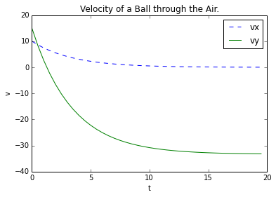 And we’ll plot this to see what it looks like:

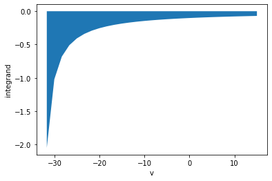 It’s helpful to plot this function to get an idea of its behavior: