Scientific Programming with Python

Installation

For your own computer you can install all of the above items as follows:

1. The package installer for Conda, Miniforge, will also install python.
• Windows:
1. Download Miniforge from https://conda-forge.org/download/.
2. Run the installer and respond to the default prompts, except as follows.
3. If you do not already have Python installed, check the box Register Miniforge3 as the system Python.
4. Check the box Clear the package cache upon completion.
5. Finish the installation by clicking the button Install.
6. To use the software, look in your Start menu, where Miniforge Prompt should show up as recently added; right-click on it and select Pin to taskbar to make it easily accessible.
7. Click on it to launch it. This is a command-line interpreter, and will display a prompt ending in >, following which you will type out commands, at the end of which you will always type the key <enter>. This interpreter is called PowerShell, but we’ll always refer to it as the Terminal or Shell for uniformity.
• MacOS or Linux:
1. Download Miniforge from https://conda-forge.org/download/.
2. Open the application Terminal. On Macs, it can be found in the folder Applications > Utilities. This is a command-line interpreter, and will display a prompt ending in $, following which you will type out commands, at the end of which you will always type the key <return> , which we’ll always refer to as <enter> for uniformity.
3. To access the downloaded Miniforge installer, type:
   
   cd ~/Downloads
4. To run the installer, type:
   
   bash ./Miniforge3-Darwin-arm64.sh
5. Run the installer and respond to the default prompts, except as follows.
6. When the installer asks Proceed with initialization?, type:
   
   yes
7. When the installer finishes and you see the $ again, close this window by typing
   
   exit
8. Open a new terminal window so that it will load the new software.
   
2. You can test your installation by typing:
   
   python
   
   which should respond with:
   
   Python 3.13.13 | packaged by conda-forge | (main, Apr 8 2026, 01:56:49) [MSC v.1944 64 bit (AMD64)] on win32
Type "help", "copyright", "credits" or "license" for more information.
>>>
   
   The >>> is a prompt for input; try typing:
   
   1 + 1
   
   Does it respond correctly?
   
   Now leave the program by typing:
   
   exit
   
3. Configure the conda channel priorities for obtaining packages:
1. To view the current channels, type:
   
   conda config --show channels
2. The Anaconda channel comes with restrictions outside of academia. To instead prioritize conda-forge, type:
   
   conda config --add channels conda-forge
3. To estabish strict channel priority, type conda config --set channel_priority strict
4. Notice that your command prompt begins with the text (base). This is the Conda default environment. We’ll now create a specific programing environment for this course, and activate it:
1. Type: conda create -n scipy
2. Type: conda activate scipy

Creating specific programming environments makes it easier to use python programs with different version requirements, and by helping avoid installation conflicts.

5. Notice that the command prompt now begins with (scipy) to indicate your current environment. Install the scipy libraries:
• Numpy: conda install numpy
• Scipy: conda install scipy
• Pandas: conda install pandas
• StatModels: conda install statsmodels
• Matplotlib: conda install matplotlib
  
6. All but the last of the packages you installed actually depend on some of the preceding packages, and they would have installed them if you hadn’t already done so. To see all of your installed packages, type:
   
   conda list
7. We will now install spyder, so it is available to the current environment.
1. Type:
   
   conda install spyder
   
   You will see a lot of information about the various packages that are required to run spyder, which is actually built with Python.
2. When the installation is finished, you can test it by typing:
   
   spyder
   
   and the program should start up.

You can leave the current environment (but not now!) with the command:

conda deactivate

Integrated Development Environments

Integrated Development Environments (IDEs) are extremely useful tools for programming, providing syntax coloring and checking, debugging capabilities, and more.

Python comes preinstalled with an IDE called IDLE (can you guess why?), but we will instead use Spyder, which has many more features and in some ways is easier to use.

There are many other Python IDEs available, see this fairly comprehensive list.

You can also just use any good programmer’s text editor (BBEdit for Mac, Notepad++ for Windows, Emacs, VIM, etc.) and run Python from the terminal, as above.

In any case, the Spyder window should open with a set of panes and toolbars that let you interact with Python:

The panes include:

• the IPython console, where you can try out various Python statements to see their effect;
• the Editor, where you can edit files that contain Python statements, and then run them to see their output in the console;
• the File explorer, which displays the locations of your Python files for easy access;
• the Variable explorer, which provides information about Python variables and their values;
• the History log, which maintains a list of previously executed Python statements.

By default there are three visible panes, sometimes with buttons that let you switch between multiple overlapping panes.

Panes can be “popped out” by clicking on the button , and then moved around into a new location or to overlap another pane.

Other panes providing additional information can be added via the menu View > Panes. If you accidentally close a pane, you can reopen it here, too.

The toolbars include:

• The File toolbar, with the usual buttons  New,  Open, and  Save to select a file to work on in the Editor;
• The Run toolbar, which lets you evaluate the Python statements in the file currently open in the Editor by clicking on the button  Run;
• The Global working directory toolbar, which lets you select the working directory that appears in the File explorer by clicking on the button  Browse a Working Directory:
  
  Note: A directory is the same thing as a folder.

Other toolbars providing additional functionality can be added via the menu View > Toolbars.

A Scientific Calculator

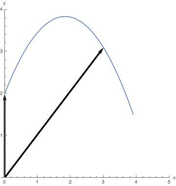
Consider the basic law of gravitational acceleration near the Earth’s surface, which applies if you throw a ball up into the air:

y = y₀ + v_y0t - ½ gt²

Here y₀ is the initial height, v_y0 is the initial speed in the vertical direction, g = 9.81 m/s² is the acceleration of gravity, and t is time.

At its most basic, Python will act like a scientific calculator and let you calculate the result of this equation by typing in particular values for these symbols and using the standard mathematical operators:

+ addition                  - subtraction

* multiplication         / division

** exponentiation

Using y₀ = 2 m, v_y0 = 15 m/s, and t = 3 s, type the following expression into the IPython console at the prompt In [1]:, and then evaluate it by typing the character <return>/<enter>:

2 + 15 * 3 - 1/2 * 9.81 * 3**2

⇒ 2.8549999999999969

The second line, the value of the expression, will appear in the console window.

There are several things to be aware of here:

• Like a calculator, you need to make sure your units match up. Since the gravitational constant is 9.81 m/s², 2 must be in meters, 3 in seconds, and 15 in m/s — but the units themselves aren’t actually typed into Python.
• The operators have different precedences, so that exponentiation will be applied before multiplication and division, which will be evaluated before addition and subtraction.
  
  If you want to change this order, you need to place parentheses () around the lower-precedence operation, e.g. (2 + 15)*3.
  
  A complete list of operator precedence can be found here.
• Within the precedence levels of addition/subtraction and multiplication/division, operations are applied left-to-right.
  
  Therefore, 1/2*9.81 is calculated exactly the same as (1/2)*9.81, while 1/(2*9.81) will produce a different value.
• Exponentiation, on the other hand, is applied right-to-left:

2**3**2

⇒ 512

(2**3)**2

⇒ 64

Try this!

Computer Numbers

Python distinguishes between integer and floating point (real) values, which you can tell apart by the presence or absence of a decimal point, e.g. 1 and 1.0 are different types of data and are stored by the computer in different ways.

You can write real values in scientific notation using the letter e to represent the ×10 (there should be no space around it):

2e-3

⇒ 0.002

This representation of real numbers should tell you where the name “floating point” comes from; we could just as easily represent this number as 0.2e-2 or 20e-4. In fact, this is how these values are stored in memory on a computer, as a pair of integers, the mantissa and the exponent.

Computer memory is structured as a set of binary digits or bits, which each have the value 0 or 1.

Bits are generally grouped in units of eight called bytes, e.g. 01110011, which form base-2 numbers that range from 0 to 28 – 1 = 255.

Often the eighth (left-most) bit of a byte is used as a sign bit, in which case the values range from –128 to 127:

Integers are defined by grouping together 1, 2, or 4 bytes, depending on the range of values desired, and interpreting them as binary numbers, as above.

Floating-point values are defined by grouping together 4 or 8 bytes, commonly called single and double precision, respectively. The available bits are split between the mantissa and exponent and their signs, 24 + 6 + 2 and 53 + 9 + 2, respectively.

The size of Python integer and floating-point values are, by default, determined by the operating system.

On newer computers (i.e. with 64-bit hardware that can transfer 8 bytes of data at once), ints are 4-byte signed, while floats are double precision.

You can tell the floating-point precision by the number of digits that Python prints out for values like 2.8549999999999969, showing all the available precision (keep in mind, though, that if the input data isn’t this precise the output won’t be, either!).

When describing data sizes, keep in mind that numbers like 1, 2, 4, and 8 will usually refer to bytes, while numbers like 8, 16, 32, and 64 will usually refer to bits.

You can explicitly force conversion of an integer to a real value with the built-in constructor float():

float(1)

⇒ 1.0

Try this!

Or go the opposite direction with the constructor int(), which truncates the fractional part of a real number:

int(9.81)

⇒ 9

Try this!

To round off to the nearest integer, instead of truncating, apply the function round():

round(2.8549999999999969)

⇒ 3

Try this!

Be aware that round()always rounds half-values, e.g. 1.5 or 2.5, to the nearest even value  — both of these will round to 2. This helps reduce cumulative errors that might occur when working with large amounts of data.

More generally, your data will have an inherent precision determined by measurement and systematic errors, and you can round calculations to maintain that precision. Simply provide round() with a second argument specifying the number of decimal places to preserve:

round(2.8549999999999969, 3)

⇒ 2.855

Try this!

Spyder provides a quick reference for Python’s built-in and library functions like round() — if you click on their name and then type <ctrl>-I (Windows) or <command>-I (Mac), its description will appear in the window Help, so that you can verify its argument format:

You can also learn about Python’s other built-in functions by typing in their names and pressing <return>/<enter>.

Warning: In Python version 3, when you divide two integers, the result will be a float if there is a fractional part:

1/2 ⇒ 0.5

But in versions 1 and 2, the result is an integer so any fractional part will be truncated, e.g.

1/2 ⇒ 0

To force truncation in any version, you can use the integer division operator //:

1//2 ⇒ 0

Variables

Just as in mathematics, assigning literal values to variables will allow you to remember their purpose and make use of them more easily.

Python lets you use variable names of any length, though they must start with a letter and afterward can contain letters, numbers, and the underscore (_). Be aware that variable names are case-sensitive, i.e. y is not the same as Y.

If you follow variables with an = sign and any value or expression such as the above, they will be assigned that value and have that type:

y0 = 2
vy0 = 15
g = 9.81
t = 3
y = y0 + vy0 * t - 1/2 * g * t**2
y

⇒ 2.8549999999999969

Try this!

Note how similar the last expression is now to the way we write the law of gravity in scientific texts.

(Also note that the IPython console doesn’t print out the values of assignments, only single variables or expressions.)

Python variables are dynamically typed, so you can redefine a variable at will, e.g. vy0 is an integer above but becomes a float with:

vy0 = 15.0

We can check the type of a variable with one of Python’s built-in functions:

type(y0)

⇒ int

type(g)

⇒ float

Try this!

A generally useful rule: if you will use the result of a calculation more than once, it’s usually a good idea to first assign it to a variable.

Variables are always pointers to areas of computer memory; they can be reassigned to other values at will, e.g.

temp = 100

temp = 200.5

The previous memory area holding the value 100 will be marked for deletion and eventually cleared when Python starts its garbage collection process.

If a variable and the memory it references are no longer needed and the latter is particularly large, it is a good idea to delete the variable manually:

del temp

If you ask for the value of a variable that has not been assigned a value or has been deleted, a name error will occur:

temp

⇒ NameError: name 'temp' is not defined

Functions

It would be useful to be able to repeat the calculation of position in Earth’s gravity for many different times without having to type out the whole expression repeatedly.

We can achieve this by packaging the statement above inside our own function definition statement:

def y(t):
    return y0 + vy0 * t - 1./2 * g * t**2

y(3.1)

⇒ 1.3629499999999908

Try this!

There are several things to be aware of here:

• The colon (:) is required to terminate the initial statement;
• All subsequent statements that are calculated as part of the function must be indented by a standard amount (4 spaces = 1 tab);
• When typing this into IPython, it will automatically indent after it sees the colon, and at the very end you need to type an extra <return>/<enter> to leave the indented level and evaluate the function definition;
• The function is aware of the earlier assignments to y0, vy0, and g, which are known as global variables;
• When the function is called with the value 3.1 in place of the argument t, the latter is replaced by the calling value everywhere it occurs inside the function, and the previous global assignment t = 3 is ignored;
• The value of the function call y(t) is the value of the expression in the return statement.
• Function calls can be used anywhere a number or variable can be used.
• The reserved words def and return have special meaning for Python, and are examples of several that must not be used for variable names.
  
  Here is a complete list of Python’s reserved words.

We can generalize this function by including multiple arguments in the definition, and we can also make g a local variable :

def y(t, y0, vy0):
    g = 9.81
    return y0 + vy0 * t - 1./2 * g * t**2

y(3.1, 2, 16)

⇒ 4.462949999999992

Try this!

Just like the function arguments, when g is defined as a local variable inside the function it will supercede any declarations outside of the function, which are known as global variables.

Local and global variables have different scopes or namespaces, and therefore are independent of each other.

Using local variables helps keep your definitions in one place and ensure they aren’t accidentally overwritten, which will make your code easier to debug.