The Basics of Using Excel |
|
Excel works somewhat differently from a word processor
like Word, and provides a powerful approach to
manipulating large amounts of data, whether quantitative
or categorical.
This tutorial covers the fundamentals
of using Excel: selecting data, editing it,
and formatting it.
In this tutorial you'll be working on a specific set of data, so
the first step is to make your own copy.
Excel files are called workbooks, and have a file type
of .xls (the older format) or .xlsx (the
newer 2007/2008 format).
- In your Web browser, visit this Web site and download its contents: https://ats.amherst.edu/software/excel/basics/stateinfo.xlsx,
and click on the button Open.
- Navigate to the downloaded file and double-click on it;
 Excel should open. Excel should open.
- Once Excel opens, the banner PROTECTED VIEW will display across the top of the file; click the button Enable Editing.
- In your Web browser, visit this Web site and download its contents: https://ats.amherst.edu/software/excel/basics/stateinfo.xlsx,
and click on the button Open.
- In the Mac Finder, open the folder Applications , then open Microsoft Office, then double-click on Microsoft Excel.app.
- Once Excel opens, click on the
menu File,
then click on the menu item Open, and navigate to the downloaded file and open it.
Microsoft Excel provides a powerful approach to
manipulating large amounts of data.
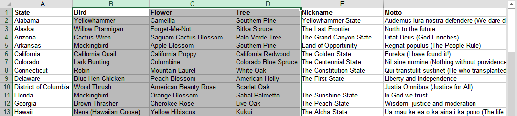
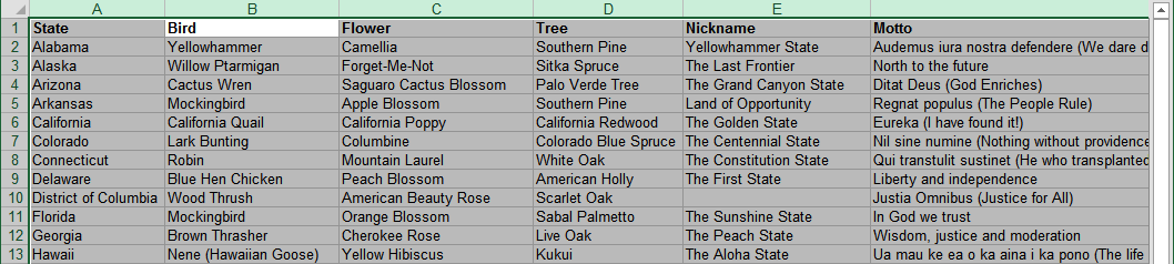
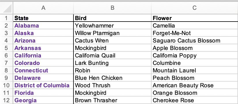
When you open an Excel workbook, it will
display a table of information, such as this
collection of the United States and some of
their characteristics:
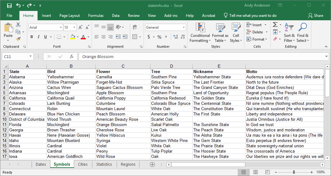
This rectangular array of data is known as a spreadsheet.
Each piece of data appears in its own cell, which are labeled
in their column headers by A, B, C,
... and in their row headers by 1, 2, 3,
....
So, you can reference Florida's state flower, the orange blossom, by
the combination C11 that describes its cell.
As you can see in the picture above, when cells are selected, they
are surrounded by a green border, and the corresponding
column and row headers are colored green.
At the bottom of the window you should see a set of tabs, here Dates,
Symbols, Cities, Statistics, and Regions.
These tabs let you choose between multiple spreadsheets stored in this
workbook.
Experiment: Click on the different tabs
to see what information is stored in this workbook's
sheets. Use the scrollbars on the right and bottom
of the window to move through the material.
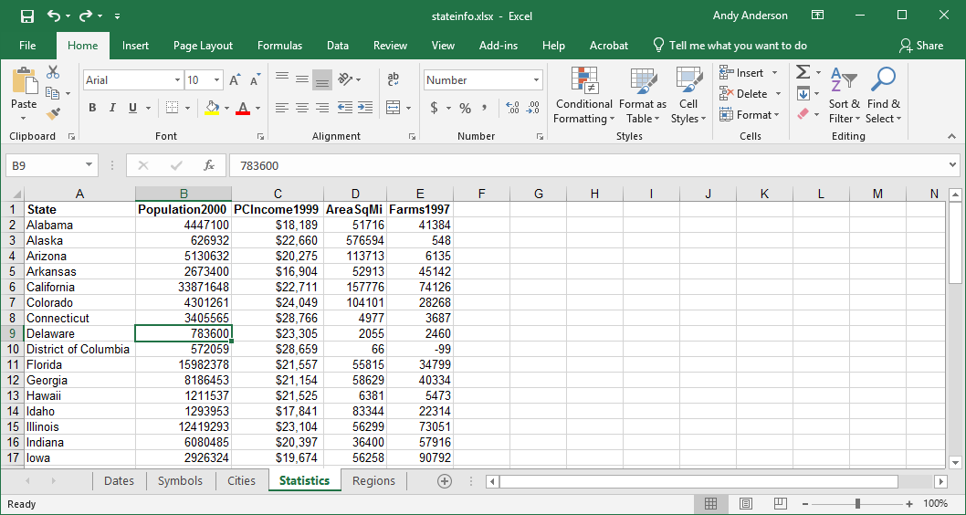
Note that data can be both categorical, as in the Symbols, Cities, and Regions sheets,
and quantitative,
as in the Dates and Statistics sheets.
By default, data that is recognized as numerical in nature (including dates and times) will be right-justified in their cell; all other data will be left-justified.
The orange blossom cell C11, being part of the sheet Symbols,
can be referenced from anywhere in the workbook
by the expression Symbols!C11. Similarly, the population of Delaware can be referenced by Statistics!D9.
Each cell in a spreadsheet is a tiny container of information, and
a little later we'll see how to edit that information.
First, however, we'll learn how to manipulate many cells all at once
by selecting them in groups, called cell ranges.
Try each of these
methods for selecting single cells:
- You can select a
cell with a single click on it (see the image above
where
C11 is selected). (Avoid double-clicking for the time being!)
- You can change the selection to adjacent cells by pressing
the arrow keys →, ←, ↑, ↓ to move in
the corresponding direction. You can also
use the keys Tab and Shift-Tab to
move right and left, respectively, and the
keys Enter and Shift-Enter to move
down and up, respectively.
- You can also move the selection to the end of
a block of contiguous filled cells by holding
down the Ctrl key and pressing an arrow key.
A single selected cell is called the active cell.
Now try each of these methods for selecting
cell ranges:
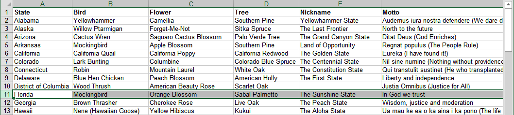
- You can select entire columns or rows of cells by clicking
on their header (e.g. on
C or 11,
respectively):
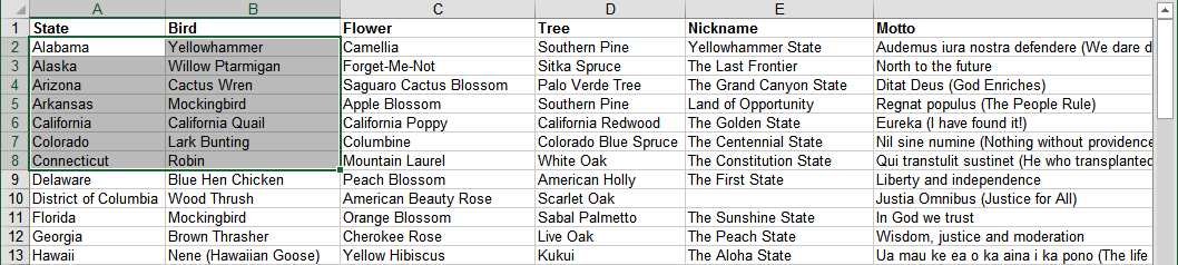
- You can select an arbitrary rectangle of contiguous cells
by click-holding and dragging across them.
Here the cell A2 was clicked on, and while holding
down the mouse button, dragged over and down to cell B8 to
produce a rectangular cell range:
- You can also select any number of adjacent
rows or columns by click-holding on their header
and dragging across them.
Here the column header B was
clicked on and dragged over to the column header D:
Notice that
in each of the previous pictures, all but one
of the cells in the range is gray; this cell
is the active cell for this range, and it
provides a reference for subsequent actions on
the range.
You can move the active cell around within the cell range using
the keys Tab and Shift-Tab to move
right and left, respectively, and the keys Enter and Shift-Enter to
move down and up, respectively. Here you cannot use the
arrow keys →, ←, ↑, ↓, which change the selection.
If you already have a cell range selected, you
can change or extend the selection in a number
of ways:
- To select everything up to and including another cell,
column, or row, hold down the Shift key and
click on the latter range.
Note that the final selection is determined only by the location
of the final range relative to the active cell
of the original selection, so some of the original
cells may be removed.
- To add an adjacent cell, column,
or row, hold down the Shift key and press an
arrow key.
Pressing the opposite arrow key will
undo this addition.
- To add everything through to the end of a block of
contiguous filled cells, hold down the the Shift and Ctrl keys,
then press an arrow key.
- To select the column or columns encompassing the selection,
hold down the Ctrl key and
then press the Space key.
- To select the row or rows encompassing the selection,
hold down the Shift key and then press the Space key.
- To select the entire surrounding block of contiguous filled
cells, in both the horizontal and vertical
directions, press the key combination Shift-Ctrl-Space (Mac: Command-A ).
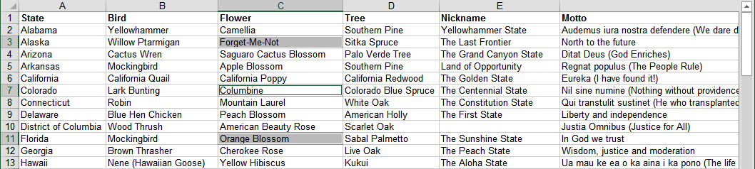
- To add a non-adjacent set of cells, columns, or rows, hold
down the Ctrl key ( Command key)
and either click on or click-hold-drag over the additional
cells, columns, or rows, as with the cells C3, C7,
and C11 below:
Whenever you want to manipulate a set of data, you can edit them collectively
as a range of cells.
Some of the common tasks you will perform including deleting cell ranges,
duplicating them, moving them, replacing them,
and inserting before them.
- In Excel,
select the range of cells you want to
delete, e.g. sheet Symbols and
column C.
- Do one of the following:
- Hold down the Ctrl key and then press
the
- key; or
- Right-click* on
the range of cells to bring
up a contextual menu, and then click on
the menu item Delete;
or
- Click on the tab Home,
then in the ribbon section Cells
click on the button
 Delete. Delete.
- On Mac Excel,
click on the menu Edit and
then select the menu item Delete….
 When a column is deleted, others to its right
are shifted left, and they are relabled so there
is no gap in the column letters, e.g. column D will
be renamed column C. When a column is deleted, others to its right
are shifted left, and they are relabled so there
is no gap in the column letters, e.g. column D will
be renamed column C.
Similarly, when a row is deleted, others below
it are shifted up, and they are relabled
so there is no gap in the row numbers.
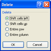
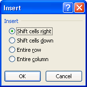
However, if the selection is a
rectangular range of cells, there will
be a question about how to fill the gap left
by the deleted cells, so you are given a few
options in a dialog that appears (shown
at the right).
Click
on one of these options and then
click the button OK.
*Note: Right mouse buttons are
not available on many Macintosh computers;
in this case, hold down the Ctrl key
and then click.
Warning: you may be used to using  Cut to
delete items, but that doesn't work in Excel;
it always requires that a cut item be moved somewhere
else. Cut to
delete items, but that doesn't work in Excel;
it always requires that a cut item be moved somewhere
else.
Duplicating and moving cell ranges are very similar, as shown in the next procedure.
In Excel, when you copy (duplicate) or cut (move)
cell ranges, the target (destination) will
always be another range of cells
you have selected (i.e. you can't select
“between” cells as when pasting text). The program therefore
distinguishes between paste (replace)
and insert (place before).
- In
 Excel,
select the range of cells you
want to duplicate
or move,
e.g. sheet Symbols and
row 10. Excel,
select the range of cells you
want to duplicate
or move,
e.g. sheet Symbols and
row 10.
- To copy or cut the cell range, do one
of the following:
- Press
the key combination Ctrl-C (Mac: Command-C)
or Ctrl-X (Mac: Command-X), respectively;
or
- Right-click on the range of cells
to bring up a contextual menu, and
then click on one of the menu items
 Copy
or Cut;
or Copy
or Cut;
or
- Click on the tab Home,
then in the ribbon section Clipboard
click on one of the buttons Copy or Cut.
- On Mac Excel or in Google Sheets,
click on the menu Edit and
then select one of the menu items Copy or Cut.
- The cell range you selected is now highlighted with a marquee;
if you change your mind and don't want
to complete this procedure, you can press
the Esc (escape)
key any time before the final step to
cancel.
- Select a target cell range; it's best
to choose the same kind as
the original: a rectangular cell range,
column range, or row range.
Warning: If the target cell range
is
smaller than the original, it will be expanded
to match during the next step, potentially
wiping out adjacent data.
- Now either:
- Replace the
target cell range by doing one of
the following:
- Press
the key combination Ctrl-V key
(Mac: Command-V);
or
- Right-click
on the target to bring
up a contextual menu, and
then click on the menu
item
 Paste;
or Paste;
or
- Click
on the tab Home,
then in the ribbon section
Clipboard click
on the button Paste.
- On Mac Excel or in Google Sheets,
click on the menu Edit and
then select the menu item Paste.
If the original cell range is
smaller than the target, it will
be duplicated to fill it.
- Insert before
the target cell range by doing
one of the following:
- Press Shift Ctrl + (Mac: Command I);
- Right-click on the target
cell to bring up a contextual
menu, and then click one
of the menu items Insert Copied Cells or Insert Cut Cells;
or
- In
Windows Excel, click
on the tab Home,
then in the ribbon section Cells click
on the button
 Insert. Insert.
- In Mac Excel,
click on the menu Insert and
then select one of the menu
items Copied Cellsor Cut Cells.
- In Google Sheets, you cannot insert before a range; you must create a blank range as described next, and then replace it as above.
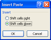 If the target is a rectangular
range of cells, there will
be a question about how to
move it out of the way to
make room for the original cells,
so you are given a few options
in a dialog that appears (shown
at the right). If the target is a rectangular
range of cells, there will
be a question about how to
move it out of the way to
make room for the original cells,
so you are given a few options
in a dialog that appears (shown
at the right).
Click on one of these options and
then click the button OK.
On occasion you may want to create a blank set of cells in the
middle of other data.
- In Excel,
select the range of cells where you
want to insert a blank cell range, e.g.
sheet Symbols and
cells C5 through
C10.
- Do
one of the following:
- In Windows Excel, press Shift Ctrl +;
or
 Right-click on the cell
range to bring up a contextual
menu, and then click on the menu
item Insert…;
or Right-click on the cell
range to bring up a contextual
menu, and then click on the menu
item Insert…;
or- Click on the tab Home,
then in the ribbon section Cells
click on the button Insert.
- In Mac Excel,
click on the menu Insert and
then select one of the menu items Cells.
- If the selection is a rectangular range of cells, there will
again be a question about how to move it out of
the way to make room for the original cells,
so you are given a few options in a dialog
that appears (shown at the right).
Click on one of these options and
then click the button OK.
As with other applications on your computer, you can undo any of these changes by pressing the key combination Ctrl-Z key
(Mac: Command-Z).
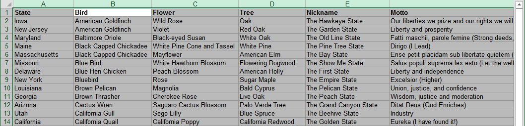
A common task with Excel is the rearrangement of data by sorting
it.
The data below is already sorted
by State name, i.e. column A:
Warning: you can sort any particular
cell range using the values in its columns, but
more commonly you will want to sort entire rows
to preserve the relative order of data within
each row. Excel will not enforce record structure
like a database program!
- In Excel,
select the range of cells you want to
sort, e.g. sheet Symbols and
columns A through F (remember the quick way?).
Warning: make sure that you select all columns that contain contiguous data so that they are sorted together, otherwise your data will be out of sync.
- Move the active cell into the
column whose values you want to sort by (or
sort by first), e.g. column B:
Tables commonly have a first line of column titles (a header) that should not be sorted, as in the example above.
Be aware that Excel will make an educated guess about whether the selected range has a header, and if it concludes so, it will automatically exclude this row from the selection when sorting, and use it to label the columns in its dialogs.
- Do one of the following:
- Click
on
the
tab Data,
then locate
the ribbon
section Sort & Filter;
or
- Click
on
the
tab Home,
then
in
the
ribbon
section Editing click
on
the
pop-up
menu
 Sort
& Filter. Sort
& Filter.
- Then:
- To sort by the values in the active
column only, click
on one of the
buttons
 Sort A to Z (Lowest to Highest)or Sort Z to A (Highest to Lowest). Sort A to Z (Lowest to Highest)or Sort Z to A (Highest to Lowest).
Be
aware that Excel's
guess about excluding
the header row will
apply here, so verify it does this correctly. If not, undo by pressing the key combination Ctrl-Z key
(Mac: Command-Z).
- To sort by the values
in multiple columns,
and/or to correct
Excel's guess about
excluding the header
row:
- Click
on the button
 Sortor the menu item Custom Sort(on Mac Excel and Google Sheets, you can also get here directly by clicking
on
the
menu Data,
then the menu item Sort…). Sortor the menu item Custom Sort(on Mac Excel and Google Sheets, you can also get here directly by clicking
on
the
menu Data,
then the menu item Sort…).
- In the dialog Sort,
the checkbox My
data has
headers may
be checked;
change this
option depending
on whether
or not Excel
was correct
in its guess.
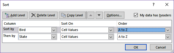
- In the pop-up
menu Column,
choose the
correct column
to arrange
your data,
e.g. Bird if
your data
has a header
row, or Column
B if
it doesn't.
- You’ll usually want to leave the pop-up
menu Sort On
set to Values, but if you’ve done conditional formatting it can sometimes be useful to sort by Cell Color.
- In the pop-up
menu Order, you can
choose a sort order:
- A to Z (alphabetical or smallest to largest);
- Z to A (reverse
alphabetical or largest to smallest);
- Custom
List…
(such as by weekday).
- If you want
to sort the
data by additional
criteria,
click on
the button Add Level and
repeat steps
iii – v,
for example
by adding State or Column
A to
put all states
with the
same bird
in alphabetical
order.
If you have a set of data that you (or others) will be repeatedly sorting, or if you want to examine subsets of the data, it’s a good idea to add a filter. It provides a separate sorting capability that will automatically maintain data within rows.
- In Excel,
select the range of cells you want to
sort, e.g. sheet Symbols and columns A through F.
Excel will always assume that the first row
of the selection contains column titles, so make sure that’s correct before the next step.
- Do one of the following:
- Click
on
the
tab Data,
then locate
the ribbon
section Sort & Filter, and click on the button
 Filter. Filter.
- Click
on
the
tab Home,
then
in
the
ribbon
section Editing click
on
the
pop-up
menu Sort
& Filter, then click the menu item Filter.
- On the Mac, menu Data > AutoFilter.
- Each column header will now have a pop-up menu button
 next to it: next to it:
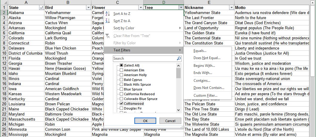
If you click on one, e.g. for the column Trees, you’ll see the available options:
- Sort A to Z (Lowest to Highest, or Ascending) — note that the column States is currently sorted this way, as indicated by its modified menu button
 . .
- Sort Z to A (Highest to Lowest, or Descending)
- Set up a filter for particular values that will be shown, e.g. for any kind of pine, click on the submenu Text Filters > Contains…, and type in “pine”.
- Pick a particular set of items, by unchecking the box (Select All)
and then checking, e.g. the box Cottonwood.

Note that the column Tree is currently filtered, as indicated by its modified menu button  . .
Warning: the filter button is sometimes hard to notice (e.g. it’s off-screen), so you may not always be aware that a table is already filtered.
When a table is filtered, any copies and cuts will only include the visible information, the hidden data will be not included.
Whenever you want to edit a particular
piece of data, you can “enter” the
cell that contains it and apply the usual editing
tools.
 Each
cell acts a bit like its own document in a word
processor, providing many of the same text-editing
capabilities for its contents. Each
cell acts a bit like its own document in a word
processor, providing many of the same text-editing
capabilities for its contents.
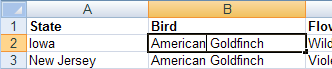
To edit the data in a cell, you must enter the
cell, which begins text-editing mode, with the usual
flashing vertical-bar cursor, as shown at the
right.
You can
enter a cell in a few ways (none of which actually use the Enter key!):
- Completely replace the
cell's contents by selecting
it and typing the new contents; or
- Position the text-editing cursor at the end of its contents
by selecting
it and:
- on Windows, pressing the key F2;
- on Mac, holding down the key Ctrl and
then pressing the key U;
- Position the text-editing cursor somewhere in its middle
by double-clicking on it.
The active cell will still be highlighted as with any
selection.
You can now use the usual methods for editing text:
- moving around by clicking the mouse or pressing arrow keys;
- typing or deleting text with the keyboard;
- selecting by double-clicking
or clicking-and-dragging with the mouse,
or pressing Shift and the arrow keys;
- cutting, copying, and pasting with menus or the keyboard.
If there is a lot of text in the cell, the cell expands when you
enter it, visually overlapping adjacent cells
that have no content.
There are a few special keys that don't work in the usual way,
but instead exit the cell and end text-editing mode:
- Enter (Return on the Mac):
move down to select the
next cell;
- Shift-Enter (Shift-Return on
the Mac): move up to select the next cell;
- Tab: move right to select the next cell;
- Shift-Tab: move left to
select the next cell;
- Ctrl-Enter (Ctrl-Return on
the Mac): keep that cell
selected;
- Esc: don't save your changes,
but keep that cell selected;
Because Enter (Return on the Mac) is used to exit a cell, if you want
to have multiple lines of text inside a cell
you must start new ones with Alt-Enter (Command-Option-Return on
the Mac).
Note: Google Sheets does, in fact, use Enter (Return on the Mac) to enter a selected cell; moving down a column is therefore accomplished with two of these keystrokes sequentially (to enter and then exit the cell).
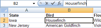 An
alternative to editing text in a cell is to use
the formula
bar; it is visible directly above the column headers. An
alternative to editing text in a cell is to use
the formula
bar; it is visible directly above the column headers.
The formula bar provides a little more room to see what you are
typing without overlapping adjacent cells, but
otherwise works the same way as editing in a
cell.
To edit text in the formula bar, you must first select the cell
and then click once anywhere in the formula bar.
The formula bar also provides alternative buttons  and and  that,
respectively, save or cancel changes to the cell. that,
respectively, save or cancel changes to the cell.
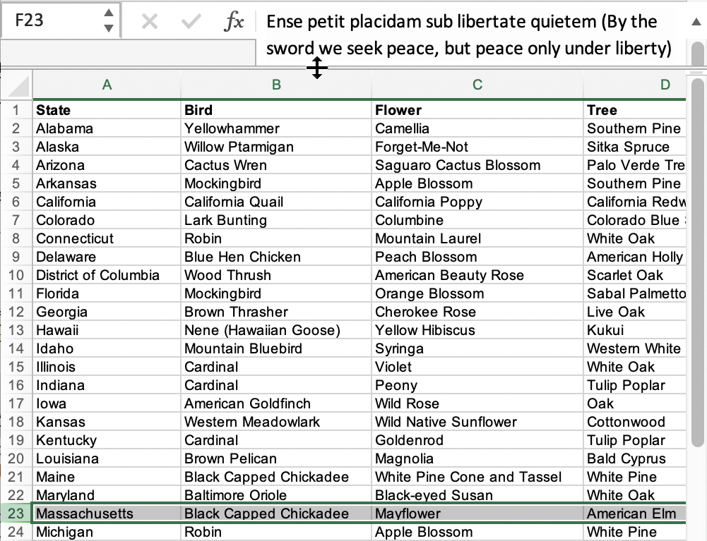 You can expand the size of the formula bar to see multiple lines of text by pointing the cursor at its bottom boundary, and when the cursor becomes a two-way up-down arrow You can expand the size of the formula bar to see multiple lines of text by pointing the cursor at its bottom boundary, and when the cursor becomes a two-way up-down arrow  , clicking and dragging the boundary. , clicking and dragging the boundary.
Excel provides many ways to format data, which can improve understanding
of its structure and characteristics.
Formatting Cells
There are numerous was to format cells; here are a few of them.
- To make sure cells are just wide enough to see everything in them, select
columns or rows containing them and then autofit them by double-clicking on the bottom boundary of the row number or the right boundary of a column letter.
- The height of rows can also be adjusted by pointing the cursor at the bottom boundary of the row number, and when the cursor becomes a two-way up-down arrow , clicking and dragging the boundary.
You can also be precise by menuing Home > Format > Row Height… and typing the number of points (e.g. for 10-point text the default is 13-point height). Then click the button OK.
- Similarly, the width of columns can be adjusted by pointing the cursor at the right boundary of the column letter, and when the cursor becomes a two-way left-right arrow
 , clicking and dragging the boundary. , clicking and dragging the boundary.
You can also be precise by menuing Home > Format > Column Width… and typing the number of characters (roughly). Then click the button OK.
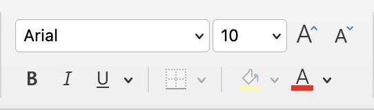  To change the font face, size, style, or color in particular cells, rows,
or columns, select them and then menu Home followed by Font, Font Size, font style like Bold or Italics, or Font Color. To change the font face, size, style, or color in particular cells, rows,
or columns, select them and then menu Home followed by Font, Font Size, font style like Bold or Italics, or Font Color.
Here you can also change the background color with the button Fill Color.
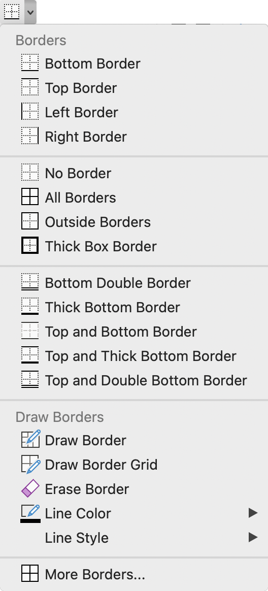
- You can also add borders to particular cells. First select them, and then menu Home and click on the button Borders.
You can then choose from different sides, All Borders, Outside Borders only, or No Borders to clear them.
You can also choose Line Style for dashed, thick, and double lines, and Line Color.
- Changing fonts and using borders helps to distinguish one group of cells
from the others:
The Representation of Numbers
One other aspect of "formatting" in Excel is the way that numbers
are represented.
- The representation of numbers will depend on what they are used for, common
formats for that purpose, and the precision one desires.
For example, the same number might have the following purposes:
- raw: "0.64"
- currency: "$0.64" (U.S. Dollars)
- time: "3:24 PM" (a fraction of 24 hours)
In addition, each of these might be written in different formats:
- raw: "6.4E-01" (scientific notation) or "64%" (percentage)
- currency: "64¢"
- time: "15:24" (military time)
Finally, we can choose the precision with which we wish to display numbers,
whether greater or smaller:
- raw: "0.6417" or "0.6"
- currency: "$0.642" or "$1"
- time: "3:24:03 PM" or "3 PM"
In all cases, the value of the number as stored by Excel is the same, only
the way it is represented is different.
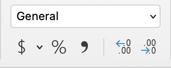 The basic formats can be selected by menuing Home and then menuing Number Format, or click on the related buttons for currency $, percentage %, and precision. The basic formats can be selected by menuing Home and then menuing Number Format, or click on the related buttons for currency $, percentage %, and precision.- The General representation is the default; it makes no assumptions, displaying
data as originally entered.
General does, however, right-align recognizeable numbers and left-align other
text.
- All of the various representations and more can be selected and designed by menuing Home > Format > Format Cells…:
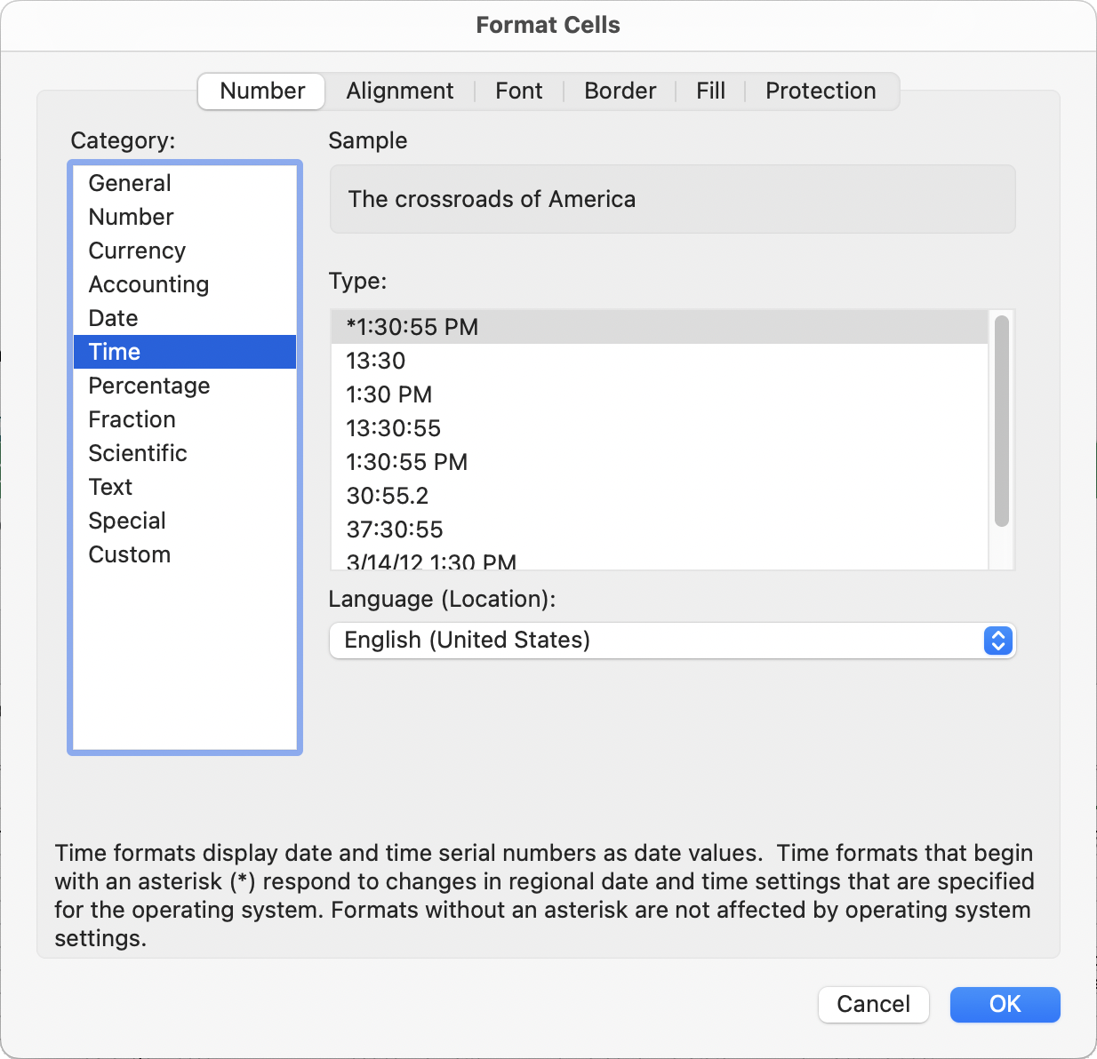
|