Geographic
data is commonly in the form of rasters, such as scanned maps, aerial or satellite photos, and
elevation grids.
Geographic raster
images have some basic features but still come
in a wide variety of formats, which are used
for specific purposes.
The Spatial Location of Raster Data
Recall that raster data, such as orthophotos or scanned maps or elevation
models, consist of a grid of pixels
whose values say something about the surface
of the Earth:

Like vector data, the raster data used by GIS will always be defined
in one particular spatial reference, where it
is a rectangular grid.
However, raster data must also
provide the following information relative to
the coordinate system of the spatial reference:
- The location of one pixel (e.g.
the center of the upper-left pixel);
- The size of its pixels, e.g. meters or
degrees, which will be either
square (usually) or rectangular (rarely);
- The amount of rotation of the raster relative to the easting
and northing directions.
This transformation information allows the position of
every pixel to be calculated and correctly displayed
relative to other data, and such rasters are
said to be georeferenced.
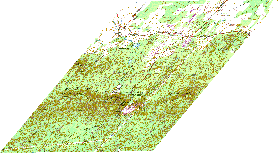
Not surprisingly, when a raster is reprojected to another spatial
reference, it will appear with a distorted shape:
|
|
Massachusetts State
Plane |
Sinusoidal |
The transformation information is stored in a number of
ways, such as a separate world
file, commonly
provided on the Internet for georeferenced rasters,
e.g. .tfw.
Unfortunately
the world file format does not also include the
spatial reference, so you must look for that
information separately, as an associated .prj
file
or as a textual description that you must incorporate
in the
same way as for vector data.
Both types of information will be stored in a .aux file, if that’s available.
The Representation of Pixel Data
 Computer and digital television screens are based on a physical grid of picture elements or pixels, each of which is a triplet of the primary colors red (R), green (G), and blue (B). Computer and digital television screens are based on a physical grid of picture elements or pixels, each of which is a triplet of the primary colors red (R), green (G), and blue (B).
The pixels are close enough together that they are visually merged, and the mixture is perceived by the brain to be one of the many colors that are visible to the human eye.
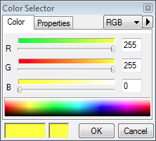  For example, equal amounts of red and green with no blue produces yellow (see the color selector at the right). Equal amounts of all three are a shade of gray. In particular, when all three are zero, the color is black, and when all three are their maximum value, the color is white. For example, equal amounts of red and green with no blue produces yellow (see the color selector at the right). Equal amounts of all three are a shade of gray. In particular, when all three are zero, the color is black, and when all three are their maximum value, the color is white.
Current digital technology usually describes each of the three values by an integer between 0 and 255, allowing the display of a total of 2563 = 16,777,216 colors. These provide a good representation of the colors that the eye can see (though this is not the entire gamut of color).
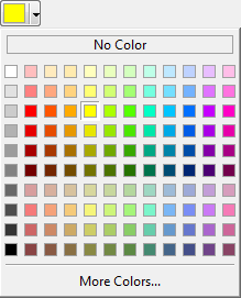
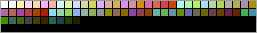
Wherever ArcGIS lets you choose a color, it will provide a palette of common colors, shown at the right, but it also lets you click on the button More Colors… to bring up the dialog Color Selector, letting you individually select the RGB values.
Raster data is stored in a number of different formats that may or may not explicitly include color information. Some of the more
common formats are:
  Color
Map or Indexed
Color: Each grid cell has a single value that is
an index into a palette of colors stored
with the raster: Color
Map or Indexed
Color: Each grid cell has a single value that is
an index into a palette of colors stored
with the raster:
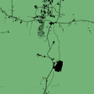
Besides limited-color
printed materials, such as the scanned topographic
map to the right (original source the U.S. Geological Survey), these values may also represent
categorical data such as impervious surfaces (far right).
If a color map is not provided with the raster, ArcGIS lets you assign colors randomly with discrete colors or to your choice of colors with unique values.
  Grayscale:
A single value that is commonly displayed
using a mathematically defined ramp ranging
between black and white: Grayscale:
A single value that is commonly displayed
using a mathematically defined ramp ranging
between black and white:
0  255 255
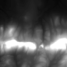
Such
a ramp is used for “black-and-white” photographs
as well as other data.
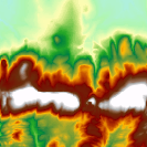
Non-photographic data could also be displayed
with a color ramp such as
0  255 255
which is commonly used for elevation.
  RGB:
A triplet of values that is displayed on
your computer screen as a visually merged
color: RGB:
A triplet of values that is displayed on
your computer screen as a visually merged
color:
| Red: |
0  255 255 |
| Green: |
0  255 255 |
| Blue: |
0  255 255 |
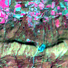
This
format is used for color photographs, along
with satellite imagery that may substitute
another wavelength of light such
as infrared, known as Color-Infrared (CIR).
The number of values assigned to each pixel is referred to as
the number of bands or channels. Multispectral
satellite imagery can have seven or more bands
per pixel, but computer display technology will
show at most three of them at once.
The values used for each pixel band may be one of several numeric
types:
Raster Pixel Types
| Pixel Type |
Pixel Depth |
Minimum Value |
Maximum Value |
| Unsigned Integer |
8 bit = 1 byte |
0 |
255 |
| |
16 bit = 2 bytes |
0 |
65535 |
| |
32 bit = 4 bytes |
0 |
4294967295 |
| Signed Integer |
8 bit = 1 byte |
-128 |
127 |
| |
16 bit = 2 bytes |
-32,768 |
32,767 |
| |
32 bit = 4 bytes |
-2,147,483,648 |
2,147,483,647 |
| Floating Point (Real) |
32 bit = 4 bytes |
-3.4
x 1038 |
1.2
x 1038 |
| Double Precision (Real) |
64 bit = 8 bytes |
-2.2
x 10308 |
1.8
x 10308 |
Generally speaking, the greater the depth, the larger the file
size of the raster, so smaller depths are used
when possible.
For example, if you have an elevation range that varies between sea
level (0 m) and 200 m, and you don’t need fractional
values, you could use one-byte unsigned
integers.
If you have a color photograph, the three RGB channels will need
at least three integer bytes; but because of
the power-of-two design of computer architectures,
they are commonly stored as a four-byte quantity.
The fourth byte will sometimes hold information about a pixel’s degree
of
transparency (or its inverse, opacity); it is
then known as an alpha channel.
For most imagery formats ArcGIS can view the individual color channels.
When opening such images, ArcMap and ArcCatalog
treat them as “folders” that open up to list
Band_1, Band_2, …. So if you want to
view the combined format, you can’t double-click
on the file, you need to click on it
once and then click the button Add.
Often a rectangular raster will include pixels that cover locations
that can’t be assigned actual values, e.g. in
an elevation data set that might lie over water.
Such pixels are typically assigned a value or
value combination that is understood to represent NoData.
If ArcGIS can determine what that “color” is, it will display
it as completely transparent (this special value
may be stored in an associated .aux file).
Rasters may be stored in a number of different
formats, which may or may not be compressed to save
space. The greatest compression is usually achieved
by using a lossy
compression format that will
not perfectly reconstruct the original data.
Raster File Formats
| File Format |
File
Extension |
World File
Extension |
Pixel Type(s) |
Compression |
Description |
| Windows BitMaP |
.bmp |
.bpw, .aux |
Colormap
Grayscale
RGB |
None (usually) |
The standard Windows image
format, very basic. |
| Graphics Interchange Format |
.gif |
.gfw, .aux |
Colormap |
Lossless |
A compressed image format
that is commonly used on the Internet
for images with simple colors and structures,
e.g. line drawings and simple scanned maps. |
| Portable Network Graphics |
.png |
.pgw, .aux |
Colormap
Grayscale
RGB |
Lossless |
A compressed image format
that is replacing .gif on
the Internet due to its better compression
and more flexible pixel types. |
| Tagged Image File Format |
.tif, .tiff |
internal
.tfw,
.aux |
Colormap
Grayscale
RGB |
Optional lossless |
Commonly
used for photographic
work as well as scientific imaging,
its use on the Internet is uneven due
to its many variations.
A new version of the format, GeoTIFF,
embeds transformation information in
the TIFF header. |
| Joint Photographic Experts
Group |
.jpg, .jpeg |
.jpw, .aux |
Grayscale
RGB |
Lossy (can be lossless) |
An
open standard that is commonly
used on the Internet for photographs
and other images with many gradations
of color. |
| Joint Photographic Experts
Group 2000 |
.jp2 |
.j2w, .aux |
Grayscale
RGB |
Lossy (can be lossless) |
A newer open standard
that
stores multiple resolutions (scales).
It is not yet completely supported on
the Internet. |
| Multiresolution Seamless
Image Database |
.sid |
internal
.sdw
.aux |
Grayscale
RGB |
Lossy (can be lossless) |
A proprietary format that
stores multiple resolutions (scales).
Supported on the Internet only via web
browser plug-in. |
| GRID |
None |
.aux |
Grayscale
RGB |
Lossless |
ESRI’s proprietary image
format, not supported
on the Internet. |
The .aux format is ArcGIS-specific, so it will
be less common even though it’s more convenient,
including both transformation and projection
information. If present it will take precedence
over a world file.
In addition to the auxiliary files, another associated
ArcGIS file you may come across is the pyramid file,
with file extension .rrd. It holds lower-resolution
versions of the original image to facilitate
rapid display when it’s viewed at smaller
scales. Multi-resolution files such as JPEG2
and MrSID include pyramids as part of
their definition. When you add other formats
lacking a pyramid file to a map, ArcGIS will
ask if you want to build one; generally
this is a good idea.
ArcGIS also stores statistics information for
images in .xml files.
Rasters are far more prevalent
on the Internet than other formats such as shapefiles
or even XY tables, because they are often
images that can be directly viewed. Make sure
to also download associated world files, projection
files, et al.!
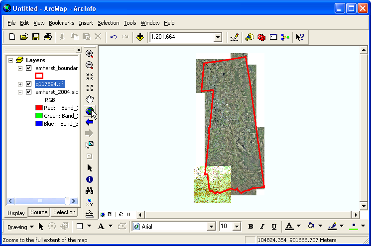
- In
 ArcMap,
in the Table of Contents,
double-click on the raster of interest,
e.g. ArcMap,
in the Table of Contents,
double-click on the raster of interest,
e.g.  amherst_2004.sid , amherst_elevation.tif, or q117894.tif. amherst_2004.sid , amherst_elevation.tif, or q117894.tif.
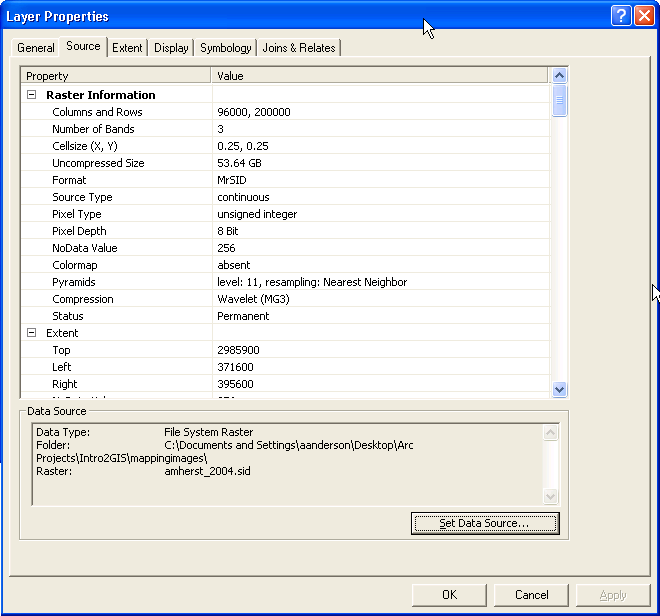
- In the dialog Layer Properties,
click on the tab Source.
- Read the table Property | Value:
- In the section Raster Information,
you should note the following:
- The number
of Columns and Rows in
the raster (in this example,
they are equal so it’s
square)
- The Cellsize (X,
Y) (pixel size) in the
units of the coordinate
system (in this example,
it’s again square).
- The file Format;
- The Number of Bands per
pixel;
- The Pixel Type and Pixel Depth;
- If a Colormap is used;
- If a NoData value is assigned;
- If Compression is
used.
- Scrolling down to the section Spatial Reference,
you should note what that is,
and also its Linear Unit (if
it has one).
- Scrolling up to the section Extent,
note the distance the raster
covers in each direction.
- Click on the button OK to dismiss the dialog.
Exercise: How does
the other raster differ?
ArcGIS will commonly display rasters in a non-uniform manner, which is often the best way to make their variations more visible, but is not always the best approach.
Visualizing the Data
The different values of the cells in a raster can vary dramatically, often in a way that is hard to visualize on a computer screen. This is because
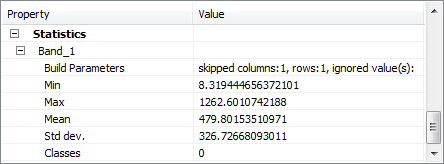 ArcGIS will usually analyze the statistics of the cell values to determine the best way to display the data. For each band, the statistics include: ArcGIS will usually analyze the statistics of the cell values to determine the best way to display the data. For each band, the statistics include:
- Minimum value;
- Maximum value;
- Mean value, which is an estimate of the middle (symbolized by μ);
- Standard deviation, which describes how the values are distributed around the mean value (symbolized by σ).
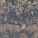
These values are included in the source properties described in Procedure 1, as in the example here for the layer amherst_elevation.tif, whose units are feet (though this must be determined from the layer’s metadata).
The statistics can be displayed and visualized by looking at the histogram of the values.
- In ArcMap,
in the Table of Contents,
double-click on the raster of interest,
e.g. amherst_elevation.tif.
- In the dialog Layer Properties,
click on the tab Symbology.
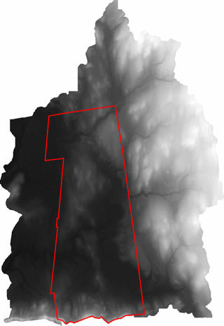
- In the list Show:, if it’s not already selected, click on the symbolization Stretched, which refers to a translation of all possible values in the raster to a particular color ramp, which by default for a single-band raster is grayscale:
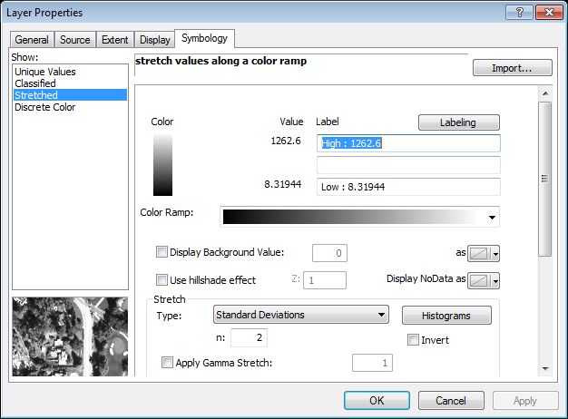
The Stretched dialog will display the minimum and maximum values in the raster, which in this case represent feet of elevation.
To be visible, a set of raster values must be stretched between black and white. ArcGIS provides a number of different methods to stretch values, and by default uses a Type: of Standard Deviations.
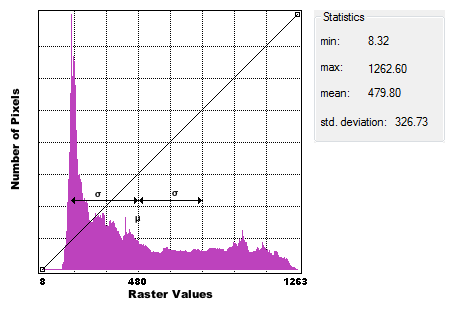 Click on the button Histograms, and the distribution of raster values will appear in a new window: Click on the button Histograms, and the distribution of raster values will appear in a new window:
- All elevation values along the horizontal;
- The number of pixels with a particular elevation along the vertical.
As you can probably tell from the raster image above, there are more low-elevation (darker) values than high-elevation (lighter) values in the raster, and this is represented in the histogram, which skews towards the lower values.
Additional statistics, the mean value μ and standard deviation σ, are also shown.
By default the minimum and maximum raster values are not simply stretched between the visible values of black (0) and white (255). Instead the stretch type Standard Deviations focuses on the range between the two values μ – n σ and μ + n σ, where μ is the mean value, σ is the standard deviation around the mean, and n is a user-defined value, by default equal to 2. Any values outside of this range are folded into black and white. This has the purpose of making the region around the mean value more visible, which is most useful when the histogram values are clustered in part of the range.
In the case of this elevation raster, this means that the values
μ – n σ = 480 – 2 * 327 = –176 → minimum value (8)
μ + n σ = 480 + 2 * 327 = 1,134
are assigned to black and white, respectively, and every value in between is stretched linearly. Everything above 1,134 is also mapped to white, which slightly enhances the contrast in the lower elevations but washes out the higher elevations.
- Click on the button OK to dismiss the Histogram dialog.
- Back in the dialog Symbology, in the area Stretch, click on the menu Type:, and select the menu item Maximum-Minimum.
This option applies the stretch over the full range of the data, which is usually better when the data isn’t clustered.
You also have the option of editing the maximum and minimum values that are stretched, which is useful when you are focusing on only a portion of an elevation raster and want to bring out its detail, or have a set of rasters with different minima and maxima that you want to symbolize in the same way.
- Click on the button OK to save your changes and close the Symbology dialog.
Exercise: How does
the other raster differ?
A fuller discussion of data statistics can be found here.
Watersheds are defined by relative elevation, and
elevation data in raster format is necessary for their analysis.
 Watersheds are
regions on the surface of the Earth where
all water flows downhill to a single point on
a stream or river, or into a particular body
of water. These are known as pour points.
Watersheds are
regions on the surface of the Earth where
all water flows downhill to a single point on
a stream or river, or into a particular body
of water. These are known as pour points.
Water is an important resource that carves landscapes, fills reservoirs, and carries soil and pollutants, so determining the extent of watersheds is important for geological, agricultural, social, and political applications.
“Downhill”, of course, means from higher elevation to lower elevation,
so elevation data is required to locate watersheds.
Many
quantities such as elevation and precipitation
vary continuously across the surface of the Earth;
they are called fields.
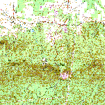
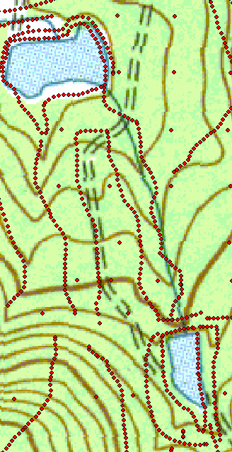
Fields are generally approximated by sampling them at specific locations,
called control points (e.g. the
red points in the image at the right), and inferring other values
in-between using geographic algorithms.
Fields can be represented by a number of formats, such as the
common visual representation in the image
to the near right of contour
lines that
have a constant elevation. “Uphill” and “downhill” are always perpendicular to these lines, and the closer together they are, the more rapid the change in elevation.
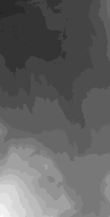
Elevation rasters such as the one to the far right of the same location are particularly useful for calculations that can
be applied uniformly to each grid cell, known as raster arithmetic,
and are therefore commonly used in watershed analysis.
- In your web browser, visit The National Map.
- Search for the area you want (it understands names like Bare Mountain, MA);
- Zoom to the extent you need;
- Click on the button Download Data at the top of the page;
- In the dialog Download options, you can choose several ways to describe the data you want, e.g. download by current map extent;
- In the dialog for USGS Available Data for Download, check on the box
 Elevation DEM Products; Elevation DEM Products;
- Click the button Next;
- A list of available rasters will appear; ArcGrid, GeoTIFF, and TIFF will be the easiest to input to ArcGIS.
The most detailed will be 1/9 arc second (~3 m), but that will also be the largest (perhaps hundreds of MB each).
Also consider the date of the rasters and if your area of interest requires the most recent or not.
Click on the name of each raster to see their extent; they often cover only part of the area you’ve selected.
Check the box next to the rasters you want to download.
- Click the button Next;
- In the panel Cart, click on the button Checkout.
- Provide your e-mail address;
- Click on the button Place Order;
- Check your e-mail for the download links they will send you.
Sources of elevation data include:
In certain areas the resolution of raster data can be as small as 3 inches or 0.25 ft per pixel.
Be aware that vertical units are typically stored only in human-readable metadata, and may differ from the horizontal units (e.g. feet vertical and meters or degrees horizontal).
The basic steps in watershed analysis are:
- Clip the raster to a small area around the watershed to reduce its size;
- Fill in any sinks in the elevation raster, which are depressions where water could collect instead of flowing downhill (often these are artifacts of interpolation from the control points or bodies of water that actually do have an egress);
- Determine the flow direction at each grid cell, which tells you how water flows downhill;
- Determine the flow accumulation at each grid cell, which lets you accurately determine the stream channels within the raster and the location of possible pour points;
- Choose one or more pour points;
- Determine which grid cells make up the watershed of each pour point.
Watershed analysis is an example of geoprocessing, a set of calculations that transform geographic data so that information can be extracted from it.
Most geoprocessing tools are found in ArcToolbox, and run in the background by default. Until you are comfortable with using these tools, it is highly recommended that you disable background processing (even with Version 10.2 of ArcGIS, background processing sometimes fails when foreground processing succeeds).
Because geoprocessing often involves a series of steps, where the the output of each step is the input to the next one, ArcGIS defines a default workspace that automatically appears as the output location in  ArcToolbox tools. However, it’s generally better to define a new one for every project. ArcToolbox tools. However, it’s generally better to define a new one for every project.
Geodatabases are collections of related content in multiple formats, specifically vector feature classes, raster datasets, and tables.
Geodatabases are the native data format for the most recent versions of ArcGIS, supplanting the older vector shapefile and raster GRID formats that are still commonly used for data interchange.
Geodatabases can be stored in database systems such as Access, Oracle, and PostgreSQL, or in a special kind of folder called a file geodatabase, which is most convenient for individual work.
ArcGIS defines a default file geodatabase, C:\Users\username\Documents\ArcGIS\Default.gdb, which is used as the default output workspace for ArcToolbox tools.
Generally, though, it’s better to create a new default file geodatabase for each project, usually in your map’s Home folder or some other accessible location.
- To work with files and workspaces within ArcMap, a number of tools are available through the
 Catalog: Catalog:
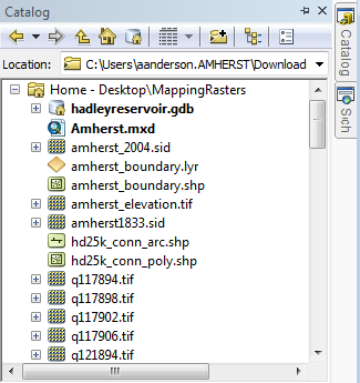 In ArcMap,
look for the vertical tab Catalog along the right edge of the ArcMap window and point at it, whence it should automatically pop out; In ArcMap,
look for the vertical tab Catalog along the right edge of the ArcMap window and point at it, whence it should automatically pop out;- If the vertical tab isn’t present, look in the toolbar Standard and click on the button Catalog.
The Catalog will appear in its own window but can be “pinned” to the right edge of the ArcMap window, which will keep it out of the way until you need it:
- Begin to drag the window and a set of “pinner” buttons will appear; move the cursor on top of the
 right-edge pinner and release. right-edge pinner and release.
- Click the button
 Auto Hide at the top of the window, so that it will go away automatically when you aren’t pointing at it. Auto Hide at the top of the window, so that it will go away automatically when you aren’t pointing at it.
- If the
 Home folder isn’t visible at the top of the catalog, save your current map document in a good location, preferably in the same folder as the data it uses, e.g. Home folder isn’t visible at the top of the catalog, save your current map document in a good location, preferably in the same folder as the data it uses, e.g.  MappingRasters. MappingRasters.
- Create a new file geodatabase by right-clicking on your home folder to bring up a contextual menu, then pointing at the submenu New
 , and finally selecting , and finally selecting  File Geodatabase. File Geodatabase.
- Give the file geodatabase an appropriate name, e.g. hadleyreservoir.gdb.
- Right-click on the new file geodatabase to bring up a contextual menu and select
 Make Default Geodatabase. Make Default Geodatabase.
Once you have your default geodatabase defined, the next step in watershed analysis is to clip your elevation raster to the area you want to study, which will speed up the process since elevation rasters are often quite large.
For this procedure you must already have an elevation raster available, e.g. the raster amherst_elevation.tif.
- You can clip the elevation raster using another raster or a polygon as a mask; only the parts of the raster that fall inside of the mask will be extracted (note: this is the inverse of how this term is usually used, where what is masked is removed).
To create a polygon mask:
- If necessary, add the toolbar Draw, by menuing Customize > Toolbars > Draw:

Dock it with the other toolbars if you want.
 In the toolbar Draw, click on the tool In the toolbar Draw, click on the tool  Rectangle; if you see another shape tool in the location shown above, click on the Rectangle; if you see another shape tool in the location shown above, click on the  menu next to it and choose Rectangle. menu next to it and choose Rectangle.- In the toolbar Draw, change the
 Fill Color to No Color and the Fill Color to No Color and the  Line Color to a bright contrasting color. Line Color to a bright contrasting color.
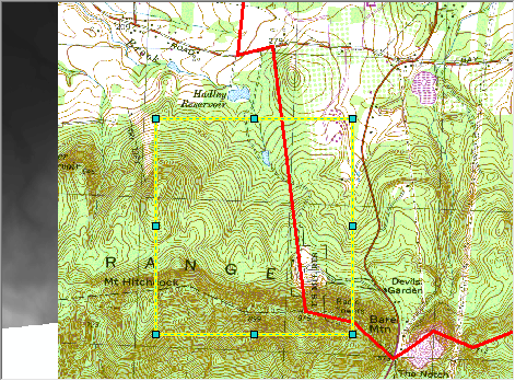
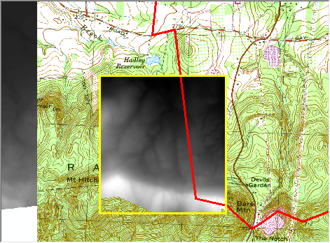
- Zoom to the area of interest, analyze the terrain to roughly estimate the watershed’s extent, and then click-and-drag out a rectangle that covers that extent — it is best to somewhat overestimate its size.
In the graphic on the right, the contours on the topographic map
help determine the approximate area over which water flows into the enclosed reservoir.
- Once you complete your drag-out of the rectangle, it will be selected and display handles (aqua boxes) around its edge; you can then adjust its position:
- You can click-and-drag the handles to reshape the rectangle;
- With the
tool
 Select Elements you can click on the outline of the rectangle (away from the handles) and drag it around; you can also move it using the arrow keys; Select Elements you can click on the outline of the rectangle (away from the handles) and drag it around; you can also move it using the arrow keys;
- If you deselect the rectangle, you can select it again with the tool Select Elements (both in the toolbar Draw and the toolbar Tools);
- If you want to redraw the rectangle from scratch, make sure it’s selected and press the key delete to remove your earlier attempt.
- To create a mask from a selected rectangle, in the toolbar Draw, in the menu Drawing, choose Convert Graphics to Features….
- In the dialog Convert Graphics to Features, the Output shapefile or feature class: is best located with your other data, e.g. in the file geodatabase
hadleyreservoir.gdb, and with a name such as area.
- Click on the checkbox Automatically delete Graphics after conversion.
- When asked Do you want to add the exported data to the map as a layer?, click on the button Yes.
The graphic will be converted to a feature class, e.g.  area, and the former will be deleted from the map and the latter added to the map. area, and the former will be deleted from the map and the latter added to the map.
- In ArcMap, turn on the Spatial Analyst extension, which provides a specialized set of tools for working with rasters:
- Menu Customize, then click on the menu item Extensions….
- In the dialog Extensions, click on the checkbox Spatial Analyst.
- Click on the button Close.
 To mask the elevation raster with a polygon or another raster: To mask the elevation raster with a polygon or another raster:
- In the window ArcToolbox, double-click on
 Spatial Analyst Tools, then on Extraction, and finally on Spatial Analyst Tools, then on Extraction, and finally on Extract by Mask. Extract by Mask.
- Drag the elevation raster, e.g. amherst_elevation.tif, from the Table of Contents into the dialog Extract by Mask and the field Input raster.
- Drag the mask, e.g. area, from the Table of Contents into the dialog Extract by Mask and the field Input raster or feature mask data.
- Choose an appropriate location for the Output raster, e.g. in the file geodatabase
hadleyreservoir.gdb, and give it a name such as elevation.
- Click on the button OK.
- When the tool has completed successfully, click on the button Close.
Once you have a raster covering the extent of the watershed, you can determine more precisely its area by analyzing the flow of water over the terrain.
For this procedure you must already have an elevation raster available, e.g. the raster amherst_elevation.tif or its clipped version, hadleyreservoir.gdb/elevation, which covers the smaller area shown above and will therefore process faster.
- In ArcMap, turn on the Spatial Analyst extension, which provides a specialized set of tools for working with rasters:
- Menu Customize, then click on the menu item Extensions….
- In the dialog Extensions, click on the checkbox Spatial Analyst.
- Click on the button Close.
- Most rasters will have some grid cells with lower elevation than any of their neighbors, which are called sinks. These are likely to be artifacts, e.g. ponds whose egress is not visible at the raster resolution.
We will therefore begin by
filling in any sinks in the elevation raster:
- Double-click on Spatial Analyst Tools, then on Hydrology, and finally on Fill.
- The dialog Fill has a number of text fields and buttons in it.
If visible, click on the button Show Help >>; it will display brief bits of information about the tool, starting with an overview and providing details about each available control (field, button, menu) as you select them.
More comprehensive information about the tool can be obtained by clicking on the button Tool Help.
- Drag the elevation raster, e.g. elevation, from the Table of Contents into the field Input surface raster.
- Choose an appropriate location for the Output surface raster, e.g. in the file geodatabase
hadleyreservoir.gdb with a name such as fill.
- Occasionally sinks are actually sinkholes that provide significant recharge for groundwater, and should not be filled; setting the field Z limit to an appropriate value can preserve these features.
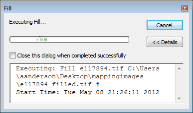 Click on the button OK. Click on the button OK.
The dialog will be replaced with another that shows how the process is Executing. When it is Completed, the output surface raster will be added to the Table of Contents. Notice that the lowest elevation is now slightly higher.- Click on the button Close.
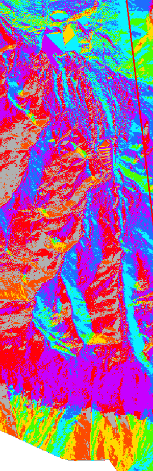
- To determine how water flows from grid cell to grid cell as it descends, calculate the flow direction:
- In the window ArcToolbox, double-click on Flow Direction.
- Drag the filled elevation raster, e.g. fill, from the Table of Contents into the dialog Flow Direction and the field Input surface raster.
 Choose an appropriate location for the Output flow direction raster, e.g. in the file geodatabase Choose an appropriate location for the Output flow direction raster, e.g. in the file geodatabase hadleyreservoir.gdb with a name such as flowdirection.- Click on the button OK.
- The dialog will be replaced by another displaying how the process is proceeding; when it is Completed, click the button Close.
The output flow direction raster will be added to the Table of Contents. The values in the raster correspond to the flow direction as follows:
|
64 — N |
|
|
32 — NW |
|
128 — NE |
|
| 16 — W |
| 1 — E |
|
8 — SW |
|
2 — SE |
|
|
4 — S |
|
Note that these directions are based on the projected coordinate system (northing and easting), not necessarily the true cardinal directions.
By default the different colors assigned to these values are chosen randomly, but if you symbolize the raster with a color-wheel ramp  the visual relationship of the directions may be more understandable. You can also relabel the symbols as shown above. the visual relationship of the directions may be more understandable. You can also relabel the symbols as shown above.
- To determine which grid cells collect the most water, in particular the stream channels within the raster, calculate the flow accumulation:
- In the window ArcToolbox, double-click on Flow Accumulation.
- Drag the flow direction raster, e.g. flowdirection, from the Table of Contents into the dialog Flow Accumulation and the field Input flow direction raster.
- Choose an appropriate location for the Output accumulation raster, e.g. in the file geodatabase
hadleyreservoir.gdb with a name such as flowaccumulation.
- Click on the button OK.
- The dialog will be replaced by another displaying how the process is proceeding; when it is completed, click the button OK.
The output flow direction raster will be added to the Table of Contents. Larger values (in white by default) are downhill, with more grid cells above them from which water could flow into them.
Note that the stream channels this tool finds may not precisely align with other data you have, such as stream shapefiles. This can be due to low raster resolution and/or limited control points, or even changing stream directions over time.
- Create a pour point for your area of interest, i.e. the lowest elevation grid cell in the area:
- Examine the flow accumulation raster to try and find the lowest point (largest value).
- In the toolbar Draw, click on the menu next to the rectangle, and choose the Marker tool. Then click on the grid cell to be used as the pour point.
- The point you choose should now be selected; in the menu Drawing choose Convert Graphics to Features…, give it an output location, e.g. in the file geodatabase
hadleyreservoir.gdb with a name such as pour_point, click on the checkbox Automatically delete Graphics after conversion, and save the result.
- In the window ArcToolbox, double-click on the tool Snap Pour Points to create a raster with the pour point(s) in the best location.
- Determine the watersheds:
- In the window ArcToolbox, double-click on the tool Watershed and fill it in.
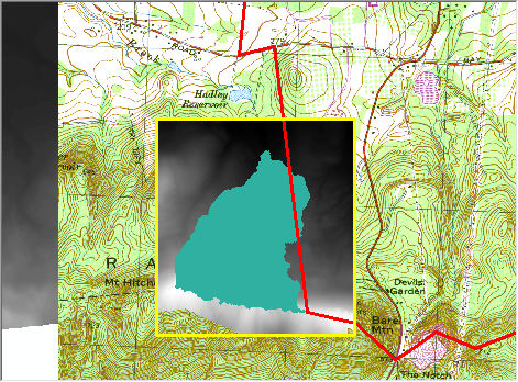
- You can determine the area of the watershed by looking at its dialog Properties and tab Symbology; by default the watershed will be colored by unique values, and the number of ”1”s present is the number of pixels.
Then switch to the tab Source where you can determine the raster’s Cell Size and Linear Unit.
For the Hadley reservoir watershed, that’s 102,586 pixels, and each pixel is 8 ft square, resulting in an area of 102,586 x (8 ft / 5280 ft/mi)2 = 0.2355 mi2.
Traditional paper maps contain a great deal of geographic
information, so it’s important to be able to
incorporate them into GIS.
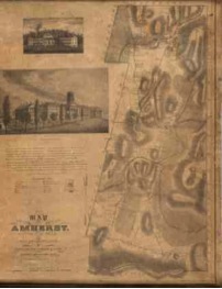
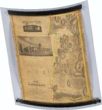
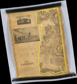
A
Map of Amherst with a View of the College
and Mount Pleasant Institution
by
Alonzo Gray & Charles
B. Adams,
Published May 1833 by
Pendletons
Lithography, Boston, MA.
(Source: The David Rumsey
Historical Map Collection, http://www.davidrumsey.com/).
Paper maps are ubiquitous,
and often they contain data that are useful
in a GIS map, e.g. as a background for other
data or to compare modern features with historical
locations.
A paper map must first
be scanned into a digital format, a now-common
procedure that
we won’t
go into here.
Scans of paper maps
and aerial photos must then be spatially positioned
to use them with other GIS data, a process
known as georeferencing.
To position the scanned map so that it aligns
with other GIS data, we can compare it with known
reference points or control points, e.g. from
an existing digital map or as collected by a
GPS receiver.
At a minimum a scanned
map must be moved to its correct geographic position,
oriented properly, and scaled to its correct
size; this requires at least two control points.
Sometimes
traditional maps are distorted; this might be
due to:
- Poor measurement;
- Intentional focus
on the relative position of features;
- Non-vertical perspective, e.g. in aerial
photos and panoramic
maps;
- Unknown projection.
Such distortions
will likely require a non-uniform scaling to
align with known features; this requires at least
six control points.
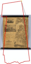
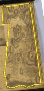
For this procedure you must already have a
scanned map available, e.g. the 1833 map
of Amherst shown above.
You must also have some reference
layers for comparison, such as boundary
files, orthophotos, or GPS points.
- Begin by adding the reference layer(s)
and scanned map to ArcMap:
- Add one or
more reference layers for
comparison, e.g.
 amherst_boundary.lyrand amherst_2004.sid (see Constructing
and Sharing Maps for
details). amherst_boundary.lyrand amherst_2004.sid (see Constructing
and Sharing Maps for
details).
- If you know or can guess
the projection of the scanned
map, change the spatial reference
of the map to match (see Mapping
Geographic Coordinate Data for
details). Otherwise, if you
don’t want to match the
reference layer(s), a
good option is Mercator,
since it is shape-preserving
and also orients north upward,
a common characteristic of
paper maps.
- Add the scanned map, e.g. amherst1833.sid.
- In the dialog ArcMap,
you will be advised that One
or more layers is missing spatial
reference information…;
click on the button OK.
- Because the scanned map has
no spatial reference information,
it will be positioned at
the origin of coordinates,
typically far from the reference
layer(s).
- Optional
Step: In the toolbar Tools,
click on the button
 Full Extent.
Viewing the full extent of
the data will likely produce
two widely separated specks,
one the correctly positioned
reference layer(s) and the
other the unplaced scanned
map. Can you tell which is
which? Full Extent.
Viewing the full extent of
the data will likely produce
two widely separated specks,
one the correctly positioned
reference layer(s) and the
other the unplaced scanned
map. Can you tell which is
which?
- To view the scanned map,
right-click on its name
in the Table of Contents and
then click on the menu item
 Zoom To Layer. Zoom To Layer.
- Examine the added map and
get a good idea of its extent
and any marked boundaries.
- Return to the original location
by right-clicking on a reference
layer’s name
in the Table of Contents and
then clicking on the menu
item Zoom To Layer.
- Z
 oom in or out from the reference
layer so that its recognizable
features roughly match those
of the scanned map. oom in or out from the reference
layer so that its recognizable
features roughly match those
of the scanned map.
- Now initiate the georeferencing process:
- If
the Georeferencing Toolbar is not already
visible, click on the menu View,
then point at the menu item Toolbars,
then click on the menu item Georeferencing.
After the toolbar appears, you
can dock it out of the way, by
clicking-and-dragging it anywhere
around the window frames.
- In the toolbar Georeferencing,
click on the menu Layer:,
then click on the menu item for
the scanned map (if
isn’t already selected — ArcGIS
will list all
image layers without a spatial
reference, and more than likely
this will be the only one).
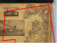
- Click on the menu Georeferencing,
and then click on the menu item Fit
to Display. The result
will look something like
the image at the right.
- This is a good time to save your
map; in the toolbar Standard,
click on the button
 Save. Save.
- You
must now add a control point that
links the same recognizable
location on the two layers, by first
clicking on it on the scanned map,
and second clicking on it on the reference
layer.
- Locations on the scanned map
are recognizable in a number
of ways:
- Point features are typically
labeled;
- Linear features such as streets,
railroads, rivers, canals,
and political boundaries
are usually labeled and have
intersections or sharp corners;
- Survey markers will often
have explicit coordinates
printed next to them;
- A graticule will
have intersections
of meridians and parallels
and explicit coordinates
at the map edges.
In the last two cases
it’s usually easiest to guess
a coordinate location on
the reference map and then
correct
it later, as described below. Warning: to
use such coordinates
you must be working in the
spatial reference of the
scanned map!
- When you have identified
a location on both maps, in
the toolbar Tools,
click on the button
 Zoom In,
and then click and drag across
both layers to draw a rectangle
containing this location on
both maps. Zoom In,
and then click and drag across
both layers to draw a rectangle
containing this location on
both maps.
- If you can’t clearly distinguish
this location on the scanned
map, drag another
small rectangle around it to
zoom in further.
- In the toolbar Georeferencing,
click on the button
 Add Control Points. Add Control Points.
 In
the scanned map, click on this
recognizable location. In
the scanned map, click on this
recognizable location.- If you’ve made a mistake,
you can hit the key Escape to
stop the link, and then continue
with Step (i).
- If you zoomed in a second time
in Step (b), then in the toolbar Tools
click on the button
 Go Back To Previous Extent. Go Back To Previous Extent.
- If you can’t clearly distinguish
the recognizable location on
the reference layer:
- In the toolbar Tools,
click on the button Zoom In,
and drag another
small rectangle around
it to zoom in further.
- In
the toolbar Georeferencing,
click on the button Add Control Points.
Notice that it still
remembers that you
have already initiated
a control point by
clicking on the scanned
map.
 In
the reference layer, click on
the recognizable location; you’ll notice that the cursor will snap to feature vertices and end points. In
the reference layer, click on
the recognizable location; you’ll notice that the cursor will snap to feature vertices and end points.
The scanned map will
now shift its position to bring
the two points into alignment.- In the toolbar Tools,
click on the button Go Back To Previous Extent to
return to the overview.
- Repeat Step 3 with a second recognizable
location; this will uniformly scale
and rotate the map to align both
the first and second points.
- Repeat Step 3 a third time using a point that’s
widely separated from
the line connecting the first two
points. This will nonuniformly scale
the map and rotate it to align all
three points. This is called a first-order
polynomial (affine) transformation.
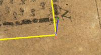 After
a fourth application of Step 3,
most likely the two points linking
the ends of the control point will no longer
be perfectly aligned, having some residual
distance represented
by a blue line, as seen to the left.
This is because there are no additional
free parameters in this transformation,
and a best
fit must
be calculated. After
a fourth application of Step 3,
most likely the two points linking
the ends of the control point will no longer
be perfectly aligned, having some residual
distance represented
by a blue line, as seen to the left.
This is because there are no additional
free parameters in this transformation,
and a best
fit must
be calculated.
- For most applications you will want
to repeat Step 3 several more times,
using points around the edge and
then throughout the middle of the
area of interest.
- To snap to intersections between two different layers, such as the boundary and street layers, it’s necessary to turn on that very useful feature; menu Customize > Toolbars > Snapping; dock the toolbar, and then menu Snapping > Intersection Snapping.
- A full description of the control
points you have set up is
provided in the Link
Table.
 In
the toolbar Georeferencing,
click on the button In
the toolbar Georeferencing,
click on the button  View Link Table. View Link Table.
The dialog Link Table should
now appear, listing each
control point link and their
starting (Source)
and ending (Map) locations.- If you click on any control point
link in the table, it will also
be highlighted in yellow on the
map.
- The link table
provides information about the
residual distance between between
the two ends of a control point
link, and the Total
RMS Error,
an average of the residuals,
which describes how far
out of alignment the entire
transformation is. We would
like it to be as small as
possible. Comparing individual
residual distances to the
total RMS error can indicate
which control points are
unusually separated. This
might be due to:
- poor surveying;
- rerouting of roads, railroads,
or canals, and the meandering
of rivers;
- deliberate abstractions,
e.g. the separation of features
to make them more distinguishable;
- bad GPS readings;
- accidental clicks.
These
points can be removed
from consideration by
clicking them in the
table and pressing the
key Delete.
- The X and Y values in the Link
Table are editable; this is most
useful if the control points
are survey markers or graticule intersections
whose values are printed on
the map, and can be typed into
the fields XMap and YMap.
- Warning: ArcMap
does not store information about
the link table, so to be able
to return to where you left off
after quitting or to restore
from a crash, you should periodically
save your table by clicking on
the button
Save… .
This will let you create a text
file storing your control points
that can be reloaded later by
clicking on the button
Load… .
- Click on the button OK
to dismiss the Link Table dialog.
 Another
way to improve the fit is to use nonlinear transformations. Their effect on the scanned
map may not always be desirable (for example,
you wouldn’t use them
on a presumably accurate map that
merely needs to be positioned). There are
several options available: Another
way to improve the fit is to use nonlinear transformations. Their effect on the scanned
map may not always be desirable (for example,
you wouldn’t use them
on a presumably accurate map that
merely needs to be positioned). There are
several options available:
- In
the toolbar Georeferencing,
click on the button View Link Table.
- In the dialog Link Table,
click on the menu Transformation:,
and then click on one of the following
menu items:
- If you have at least
six control
points, the item 2nd
Order Polynomial becomes available.
With exactly six, the Total
RMS Error will be
zero.
- If you have at least ten control points, an
additional option is 3rd
Order Polynomial . With exactly
ten, the Total RMS Error
will be zero.
- Also available with at least ten control points
is the option Spline.
It provides an exact
fit for all additional control
points, but can be very slow
due to the large number of
calculations required.
- An option available at all levels is Adjust;
it is very fast for even
hundreds of control points,
but produces discontinuities
in the image at the points’
exterior boundary.
- Click
on the button OK
to dismiss this dialog.
- Once you’re satisfied with the fit of the transformed
map, you can save it as a new raster
layer for later use. Be aware that this
process can take a while for a large
map. If you haven’t already done so, it’s advisable to disable background processing.
- It’s a good idea to first save your control
points as described in Step 8(c).
- In the dialog Georeferencing,
click on the menu item Rectify….
- In the dialog Save as,
in the text field Output
Location:, click on the
button
 Browse and
select the folder (not the file) where
you want to save the new raster. Browse and
select the folder (not the file) where
you want to save the new raster.
- In the menu Format:,
choose an output
format; for
scanned maps, JP2 or JPG is preferred,
though PNG can also be good for
relatively simple images. JPG
is the most compatible with external
applications and will typically
produce the smallest files if
you are willing to sacrifice
image quality.
- If you choose JP2 or JPG, in the text field Compression
Quality (1-100): type
a value or leave the
default (anything less
than 100 will be lossy).
- In the text field Name:,
adjust the file name to be more
descriptive, e.g. amherst1833rectified.jp2.
Don’t change the file extension
here, use Step (d) instead. Warning:
GRID-format names must have a
base that’s less than 13 characters
long.
- Click on the menu Resample
Type:, and then click on one of the
menu items Bilinear Interpolation or Cubic
Convolution(better but slower). The
option Nearest Neighbor is
best only for categorical data.
- The new raster’s cell size is initially based
on that of the scanned map, and
it’s usually best to leave it
at the default. You can, however,
reduce the file size by increasing the
cell size, by typing a new value
in the text field Cell
Size:.
- The new raster will be a rectangle in the current
coordinate system, and that means
that areas outside of the transformed
map will be set to NoData. By
default this value will be 0
(black), but you can assign those
grid cells another value (e.g.
1 — white) by filling in the
text field NoData
as:.
- Click on the button Save.
 Now review the rectified image: Now review the rectified image:
- Add the rectified image to your map, e.g. amherst1833rectified.jp2.
- The NoData areas can be made transparent
as follows:
- Double-click on the name of the
rectified image
in the Table of Contents to
bring up the
dialog Layer
Properties.
- Click on the tab Symbology;
- Click on the checkbox Display
Background Value:
(R,G,B); leave the
default color as
No Color.
- Click the button OK.
- If you use a file format other than
JPG or JP2 or PNG, ArcGIS
automatically calculates
the statistics of the
colors in the image,
and then uses them to
provide what it thinks
is a better color display. This is
almost always incorrect
for an actual image (as
opposed to rasters describing
quantities like elevation).
To turn off the use of
statistics for color
display:
- Double-click on the name of
the rectified
image in the Table of Contents to
bring up the
dialog Layer
Properties.
- Click on the tab Symbology;
- In the area Stretch,
in the menu Type:,
select the menu item
None; this allows the image’s colors to be displayed unchanged.
- Click the button OK.
- in the Table of Contents,
click off the checkbox
next to the name
of the rectified
image, e.g.
 amherst1833rectified.jp2.
You can now see that
the rectified image
matches the scanned map,
the reference layer,
and the control points. amherst1833rectified.jp2.
You can now see that
the rectified image
matches the scanned map,
the reference layer,
and the control points.
|