Not all geographic data is in a GIS-ready format. Commonly it is in the form of a table of values assigned to place names representing geographic features such as states or street addresses.
When data is associated with place names, we can join it to an existing layer providing the geography.
Geographic data ideally comes in the form of a layer, which is a set of geographic features with attributes assigned to them. We’ve already seen examples of state polygons and city points, whose attribute tables associate these features with information such as area, population, etc.
Layers also include information about the geography of the features, so they can be immediately displayed as a map, as above. Recall that the details of the geography are hidden inside the Shape field:
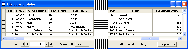
Very often, however, you may obtain or create a table of data whose only geographic connections are a set of place names that abstractly represent the geographic feature, e.g. “Massachusetts”, “Alabama”, etc. In other words, it doesn’t have a Shape field:
Such place-name data is also known as toponymic data.
Fortunately, if you have access to a map layer that defines the same geographic regions with the same names, you can join your table to that layer. Joining essentially extends its attribute table with new fields (columns), which you can then use to symbolize it, etc.
- In the Windows Explorer, navigate into the folder
 MappingPlaceNames. MappingPlaceNames.
- Locate the file
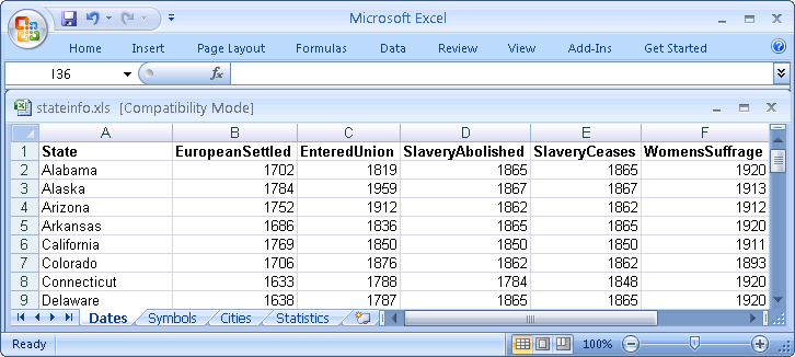
 stateinfo.xls, which is a Microsoft Excel workbook, and double-click on it to open it in Excel. stateinfo.xls, which is a Microsoft Excel workbook, and double-click on it to open it in Excel.
- Examine the workbook’s structure:
- The simple rectangular arrangement of the data;
- The initial row containing the attribute names;
- Subsequent rows each containing the data of one feature (called a record);
- Each column containing a single attribute as it varies from feature to feature (called a field).
- The worksheet names, e.g.
Dates, in the tabs at the bottom of the window. You can have many worksheets in the same workbook.
- Close the workbook.
Besides Microsoft Excel XLS or XLSX files, ArcGIS can
also read tables in several other formats:
- CSV
- Comma-separated values files are simple text
files with each
field in the table separated by commas (if
the data includes commas, the field value
must be enclosed in double quotes).
- TXT or TAB
- Tab-separated values files are also simple
text files, with each field
in the table separated by tabs.
- DBF
- dBASE files are an old database format that
are still used for Shapefile
attribute tables.
- MDB
- Microsoft Access files are a newer database
format.
All of these formats can also be read by Microsoft
Excel (but it will only open TAB files directly
if the extension is changed to TXT).
If you have data in these formats and are going
to be making any changes with Excel,
it’s generally better to first save it as XLSX;
otherwise Excel will always complain about
potential data loss when you save.
Warning: To successfully
make use of tables, their file names should start
with letters and afterwards include only letters,
numbers, and underscores.
Because the map layer and table shown above have a matching place name attribute:
- the map layer
 states.shp and its field STATE_NAME, and states.shp and its field STATE_NAME, and
- the table
 stateinfo and its field State. stateinfo and its field State.
they can be joined together, row by matching row.
Any map layer can have a table joined to it, as long as they have an exactly matching attribute that can be used to relate data for each feature.
- In
 ArcMap,
in the toolbar Standard, click on the
button ArcMap,
in the toolbar Standard, click on the
button  Add Data. Add Data.
- In the dialog Add Data, navigate into the folder with the table to be joined, e.g. MappingPlaceNames.
- Double-click on the table to be joined, e.g the Excel workbook
 stateinfo.xls. stateinfo.xls.
 In
ArcGIS dialogs, Excel workbooks are workspaces, meaning
you can open them
like folders and see an overview of
their contents. In
ArcGIS dialogs, Excel workbooks are workspaces, meaning
you can open them
like folders and see an overview of
their contents.
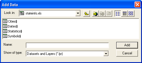
In particular, they
display their worksheets and named
regions (discussed below) as separate “files”.
Worksheets all have a $ at the end
of their names, as in the image at the
right.
If the join table is inside a workbook, double-click on the latter to see its contents, and then add the desired table to your map document by double-clicking on it, e.g. Dates$.
- After adding a table, the Table of Contents will switch to the
 List by Source view; the reason is that a table by itself is not displayable on the map, and therefore won’t show up in the List by Source view; the reason is that a table by itself is not displayable on the map, and therefore won’t show up in the  List by Drawing Order view. You wil probably want to switch back to the latter, though, since it’s simpler. List by Drawing Order view. You wil probably want to switch back to the latter, though, since it’s simpler.
 In the Table of Contents, right-click on the layer to be joined, e.g. states.shp. In the Table of Contents, right-click on the layer to be joined, e.g. states.shp.- The layer’s contextual menu will now appear; select the menu item Joins and Relates, followed by the menu item Join....
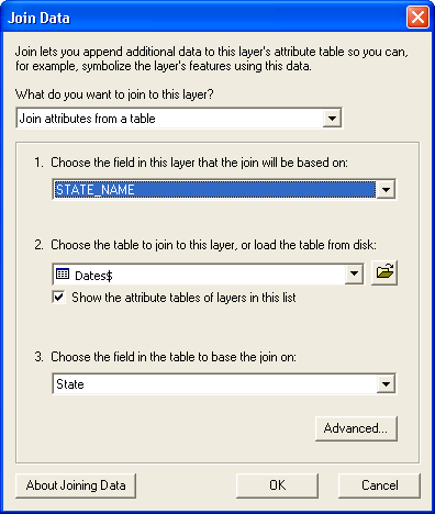
- In the dialog Join Data, in the menu What do you want to join to this layer?, make sure that Join attributes from a table is selected.
- In the menu 1. Choose the field in this layer that the join will be based on:, select the matching field in the map layer, e.g. STATE_NAME.
- In the menu 2. Choose the table to join to this layer, or load the table from disk:,
select the table to be joined, e.g. Dates$.
- In the menu 3. Choose the field in the table to base the join on:, select the matching field in the table to be joined, e.g. State.
- Click on the button OK.
Alternative: Rather than use the
“internal join” described above in Steps
1-5 and 10, you can directly join an external
table in Step 10 by clicking on the button  Browse;
this is a slightly easier one-step process. Browse;
this is a slightly easier one-step process.
However,
this “external join” has the disadvantage
that you won’t
get error messages describing incompatibilities
in your table. It also obscures the location
of the table from the ArcMap user, and if
the map document loses track of it you can’t
see its path to help you find it again to
fix the join.
To see the results of the joining tables procedure, try out the new
attributes:
- In the Table of Contents,
right-click on the layer states.shp and
select the menu item
 Open Attribute Table. Open Attribute Table.
 Examine the attribute
table’s structure: the fields from
the shapefile
are now immediately followed by the
fields from the joined table. Examine the attribute
table’s structure: the fields from
the shapefile
are now immediately followed by the
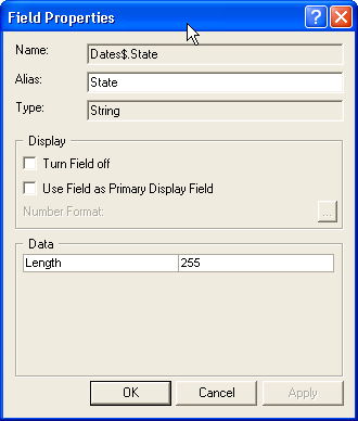
fields from the joined table.- Right-click on one of the field
headers, e.g. State,
to bring up its
contextual menu,
and select the menu item Properties… .
- In
the dialog Field
Properties, note that
the visible field name is just
an alias, and the actual field
name begins with the table name,
e.g.
Date$, followed
by a period.
This field-name prefix ensures that
there are no conflicts between fields
from the joined tables that
might have the same name.
Note that Alias: is
editable, so you
can use it to change a field name
if you think it could be more descriptive;
it has fewer restrictions on
length and characters than the actual
name.
- Close the dialog Field
Properties and then the
attribute table.
- Symbolize
the layer with one of the
quantitative fields from the
joined table.
- Save the document by clicking on
the button
 Save. Save.
Important Note: The additional fields
from the joined table have not been permanently added to the map layer,
just temporarily linked to it.
This means that if you move the table file or the map document to
some other location, the map may no longer work because ArcMap could
be looking in the wrong place for the table file.
When ArcMap can’t find a file, it places a red exclamation point ! next
to its name in the Table of Contents, and you can click on ! to
start a dialog to relink it.
Exercise: Mapping the Presidential Election
On the Internet, search for a table of the electoral votes by state in the most recent presidential election, and map them. Note that they are extensive quantities!
Nebraska and Maine are unique in that they distribute their electoral votes both statewide (2) and by congressional district (1 each). How might you represent that on your map? (Hint: Look at some of the patterns available to fill polygons in the standard symbology dialog — can you determine how they’re constructed?)
Once you’ve joined a layer and a table, sometimes you may
want to save the result as a new shapefile with
a merged attribute table:
- In ArcMap,
in the Table of Contents,
right-click on the name of the layer,
e.g. states.
- In the layer’s
contextual menu, point at the menu
item Data,
then in the submenu that appears
click on the menu item Export Data….
- In the dialog Export Data,
in the menu Export,
make sure that All features is
selected.
- Near the text
field Output shapefile or feature class:,
click on the button Browse to
navigate to an appropriate location
for the new data set, e.g. the folder MappingPlaceNames,
and give it a descriptive name, e.g. states_and_dates.shp.
Remember that file names should start
with letters and afterwards include only letters,
numbers, and underscores
- Click on the button OK.
- The dialog ArcMap will
now appear, asking if you want to
add the exported layer to the map;
click Yes or No.
One advantage of using joins is that you can more easily change the
contents of the joined table (there will be more about editing from within ArcMap later).
However, many applications such as Excel won’t allow you to edit the
table if ArcGIS also has it open.
If you aren’t changing the join attribute name, the simplest
thing to do is quit ArcMap, edit the table, and
reopen the map; the table will be rejoined as
previously defined, with the new data.
Otherwise, you’ll need to unjoin the table, remove it from ArcMap (if
an internal join), edit it, re-add it to ArcMap,
and rejoin it.
An important example of data
that is commonly joined to map layers comes
from the U.S. Census Bureau.
As another example of commonly available place name data, we’ll work with
some more census data. As you probably already
know, every ten years there is a census that
tries to obtain basic information from 100%
of the U.S. population; this is the primary
source of the data we looked at previously
in the states layer. In addition, the U.S.
Census Bureau provides many variations
of this data, as well as the results of the
annual American Community Survey that
tracks detailed information from a small
subset of the population collected every year. This data is in
tables that you must join to existing layers.
We’ll also use a type of geographic region
that you might not be familiar with, census
tracts. According to the Bureau, “Census
tracts are small, relatively permanent statistical
subdivisions of a county....Designed to be
relatively homogeneous units with respect
to population characteristics, economic status,
and living conditions, census tracts average
about 4,000 inhabitants.”
Two smaller subdivisions of census tracts
are also available, though we won’t use them
here. Census blocks are “the
smallest geographic unit for which the Census
Bureau tabulates 100-percent data....Many
blocks correspond to individual city blocks
bounded by streets, but blocks — especially
in rural areas — may include many square
miles.” Census block groups are
just that, and are the smallest region available
for some sensitive attributes such as income.
- In ArcMap,
click on the button
 New Map File. New Map File.
- Click on the
button Add Data.
- In the dialog Add Data,
navigate into the folder MappingPlaceNames.
- In the folder MappingPlaceNames,
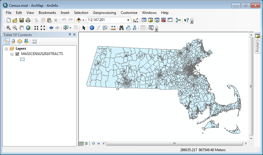
click on the file MASSCENSUS2010TRACTS.shp.
- Click on the button Add.
- Save your map document in the folder MappingPlaceNames, with a name such as Census.mxd.
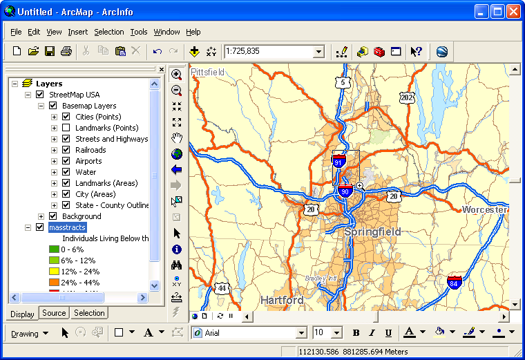
ArcMap will now display a map of the Year
2010 census tracts in Massachusetts:
If
you right-click on the layer MASSCENSUS2010TRACTS and
select the menu item Open Attribute Table,
you should see the following:
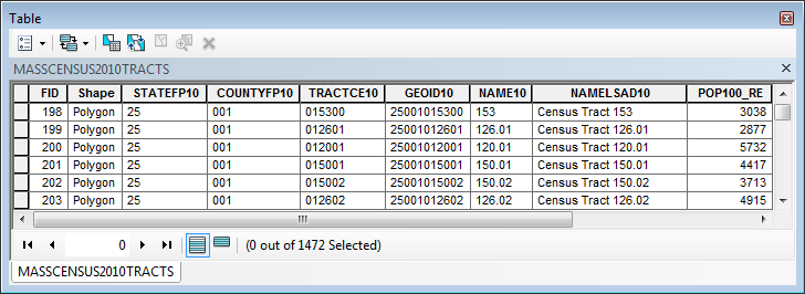
The census tracts are uniquely named by their FIPS (Federal
Information Processing Standards)
code, which begins with the two-digit
state code in the field STATEFP10 (e.g. 25 for Massachusetts), followed by the three-digit county code in the field COUNTYFP10 (e.g. 001 for Barnstable County), and finally the tract code in the field TRACTCE10 (e.g. 015300).
By combining these three together into a text string in the field GEOID10 (e.g. 25001015300), we have a unique identifier that can be used to join other
census data to this layer.
Be aware that census tracts change from decade
to decade. The Census Bureau provides cartographic
boundary shapefiles for its online data (including
other regions such as congressional districts
and metropolitan statistical areas) at http://www.census.gov/geo/www/cob/.
This particular data set actually comes from MassGIS, and includes 100% data on population in each census tract, in the field POP100_RE.
The Census Bureau also lets you download much
of their data from http://www.census.gov/. As an example, we’ll map some
poverty data from the latest American Community Survey. This survey provides much more detailed information than the decadal census, and is drawn annually from a small sample of the population.
- If necessary, start up a web
browser:
- Click on
the menu
 Start. Start.
- Point at the menu item All Programs.
- Locate your
preferred web browser,
 Chrome or Chrome or  Firefox,
and click on it. Firefox,
and click on it.
- In your web browser, visit the web
address www.census.gov.
- On the top of the web page Census.gov,
point at the menu Explore Data to let it drop down its menu, then click on the link Explore Data Main.
- On the web page Try out our new way to explore data, click on the button Go to data.census.gov (you can also just start on this page once you’re used to it).
- On the Web page Explore Census Data, click on the link Advanced Search.
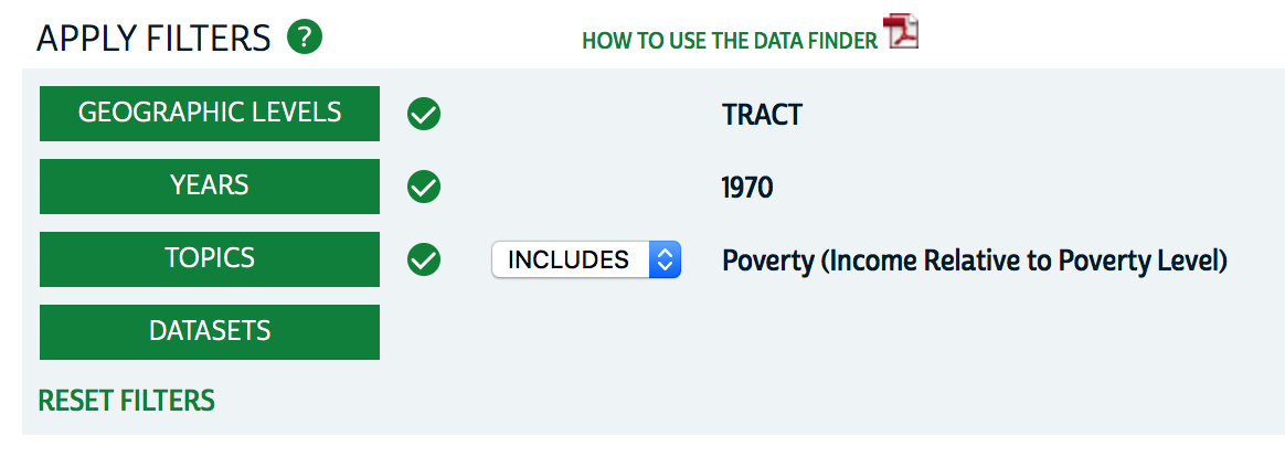
- On the left side
of the web page Advanced Search there are several ways to access census data: by topics, by geography, by years, by surveys, etc.:
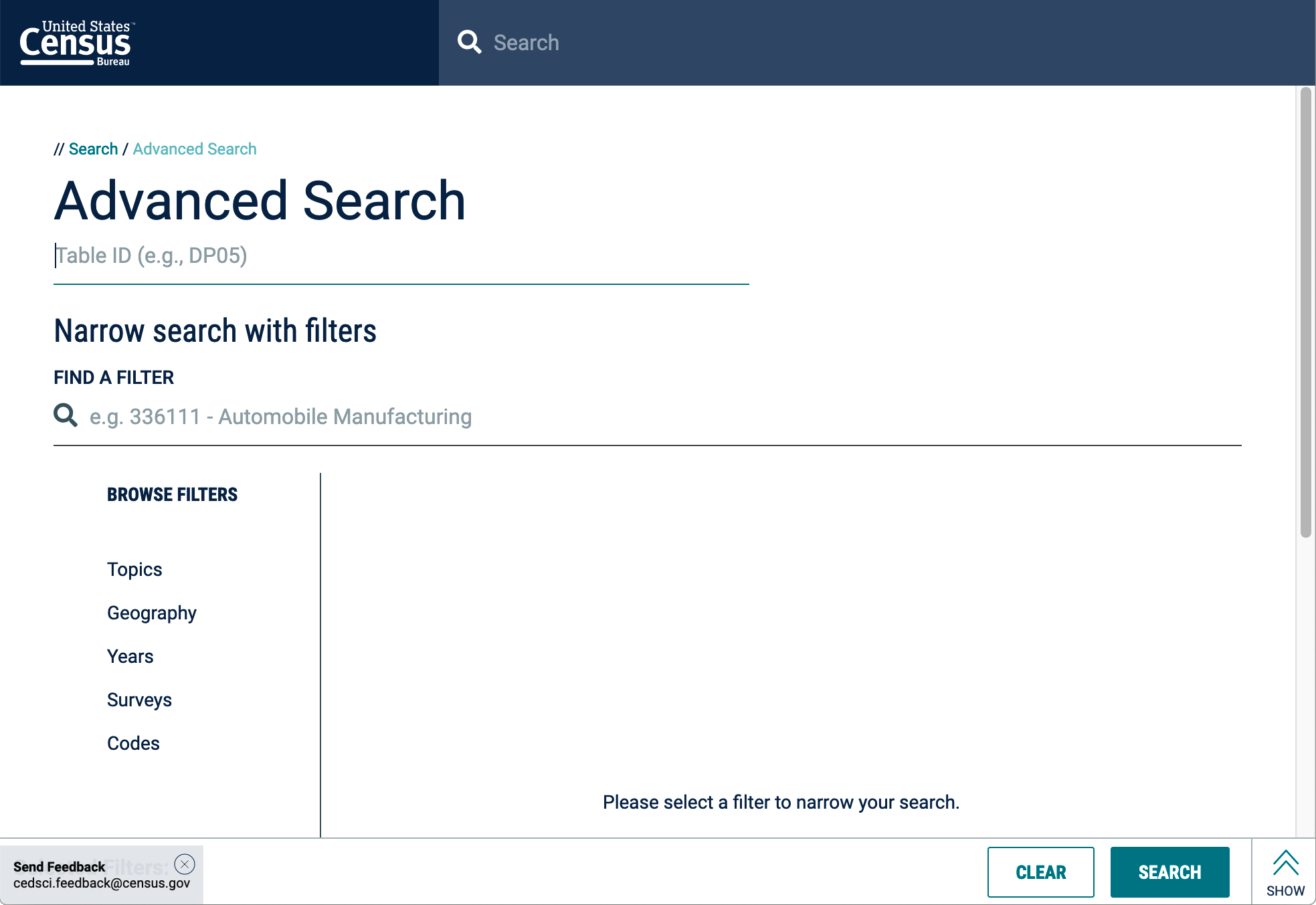
You can approach your search for data by starting with any one of these parameters, but you’ll eventually need to specify all of them, and what you find can depend on where you start, as that can narrow the availability of later parameters.
In this example we will start with geographies, then topics, then years and surveys.
 Geography must be described in multiple steps, by specifying: Geography must be described in multiple steps, by specifying:
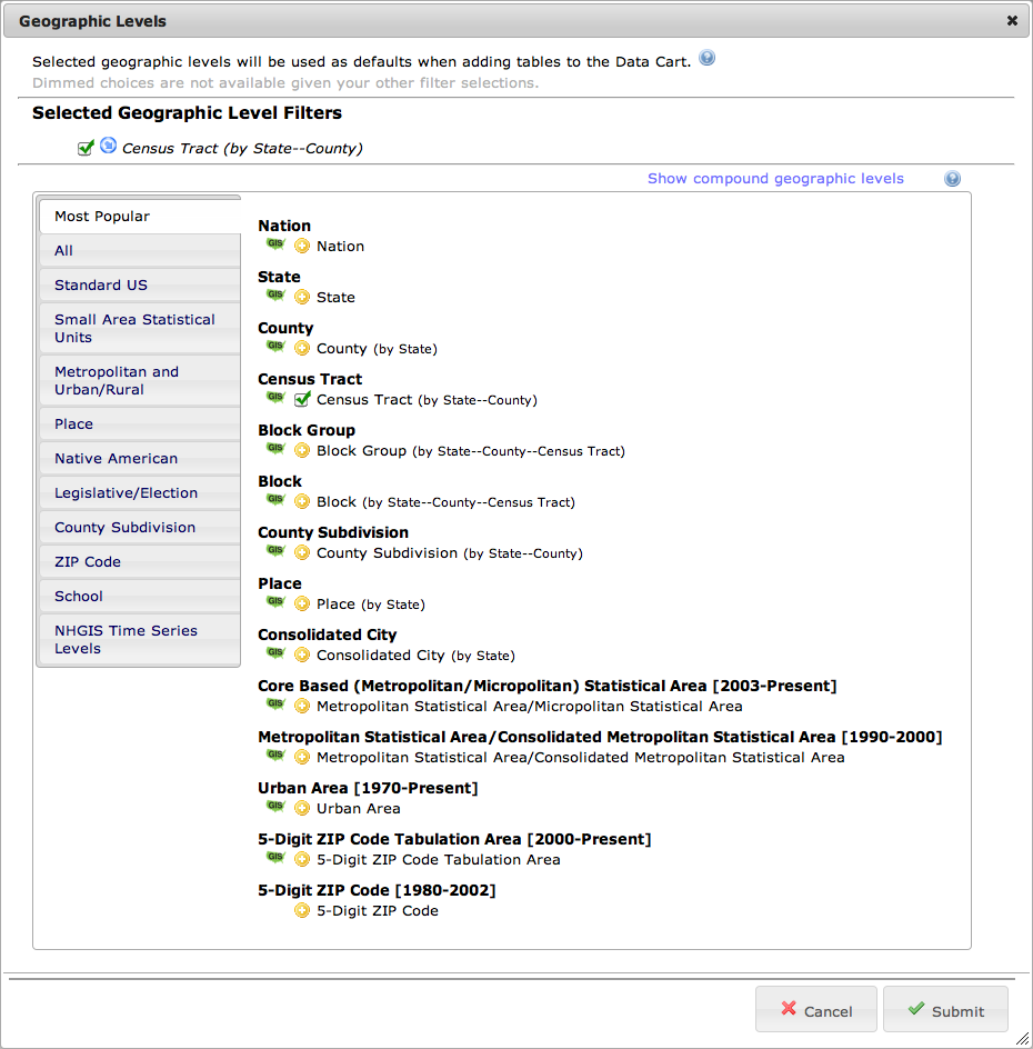
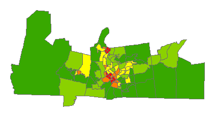
- The geographic type, the unit for which data will be summarized, for example the census tracts in the image to the right; and
- The geographic area, a larger “containing” geography within which the above data is located. It is generally specified by place name, for example Hampden County in Massachusetts, shown at the right.
In the column BROWSE FILTERS,
click on the item Geography:
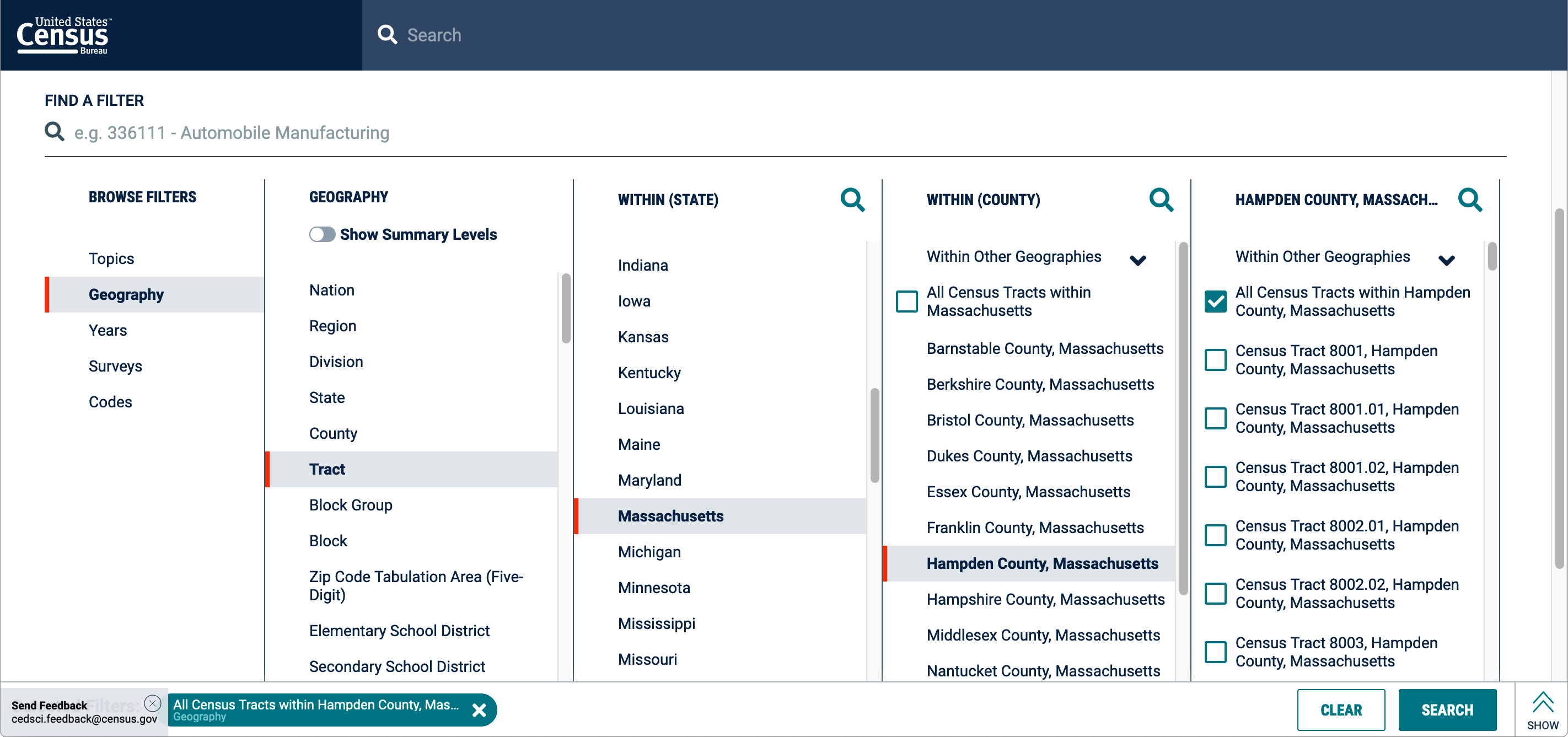
- In the column GEOGRAPHY, select, for example, Tract.
- In the column WITHIN (STATE), select, for example, Massachusetts.
- In the column WITHIN (COUNTY), select, for example, Hampden County, Massachusetts (this is the county south of Amherst, containing Springfield, Chicopee, and Holyoke).
- In the column HAMPDEN COUNTY, MASSACHUSETTS click on, for example, the checkbox
 All Census Tracts within Hampden County, Massachusetts. At the bottom of the window, a banner appears to indicate your final selection. All Census Tracts within Hampden County, Massachusetts. At the bottom of the window, a banner appears to indicate your final selection.
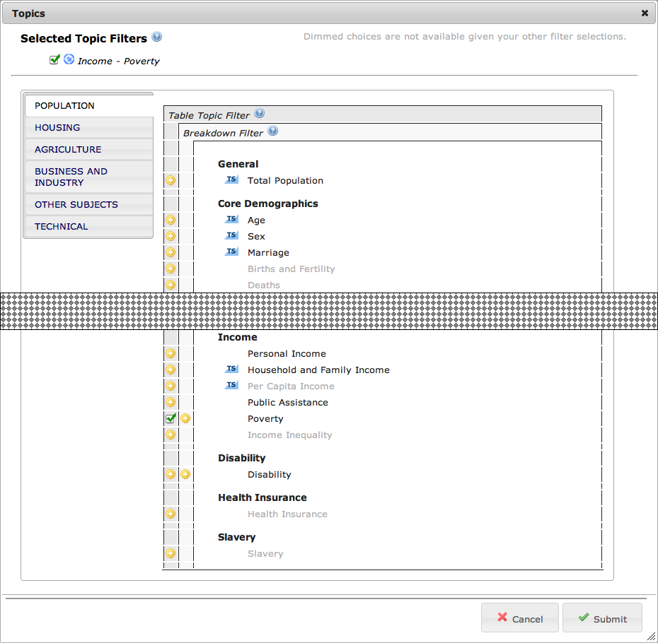
- In the column BROWSE FILTERS,
click on the item Topics:
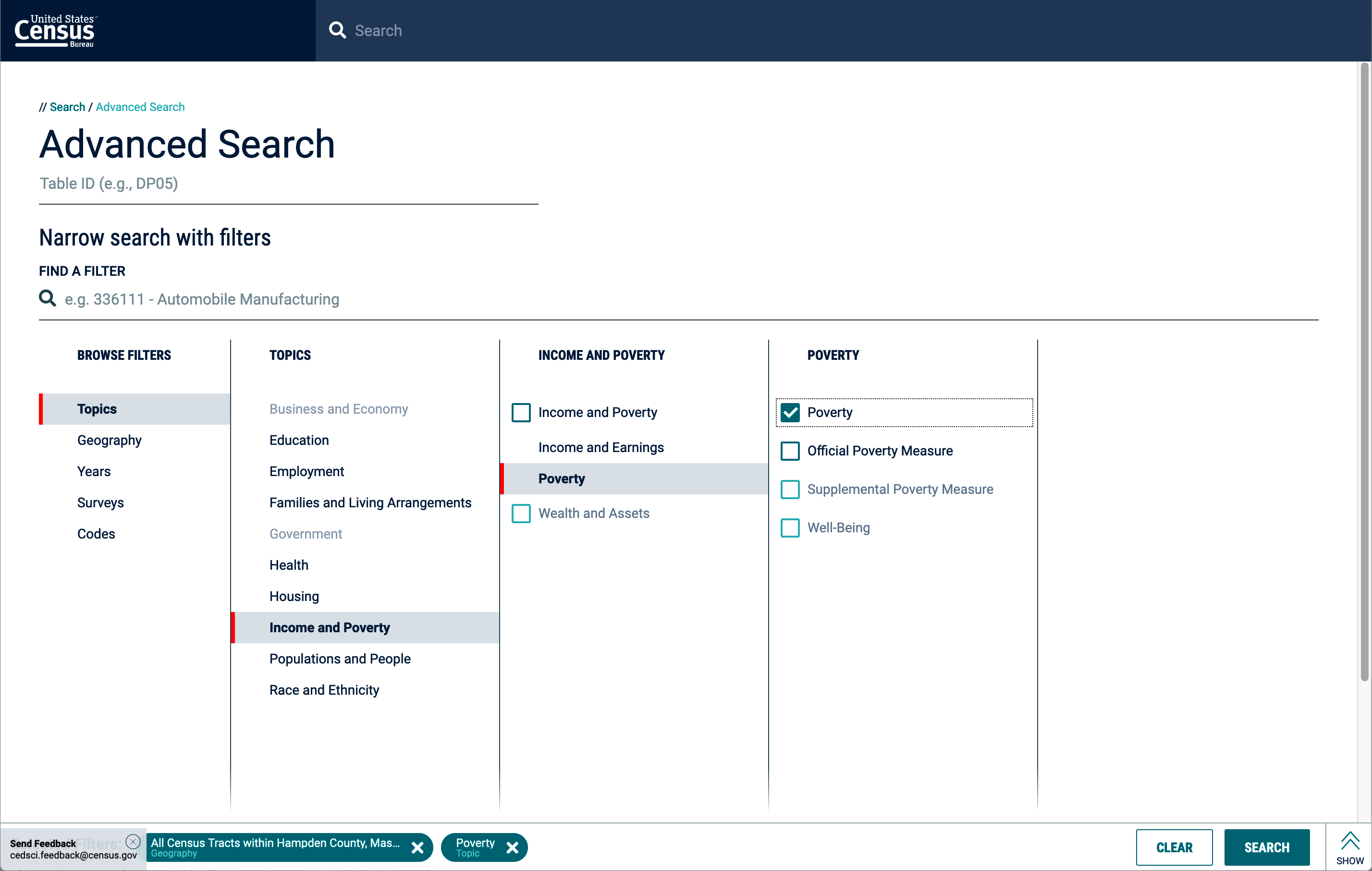
- In the column TOPICS, select, for example, Income and Poverty.
- In the column INCOME AND POVERTY, select, for example, Poverty.
- In the column POVERTY, click on, for example, the checkbox Poverty. At the bottom of the window, a banner appears to indicate your final selection.
- Finally, click on the button Search.
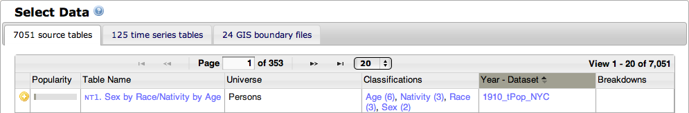
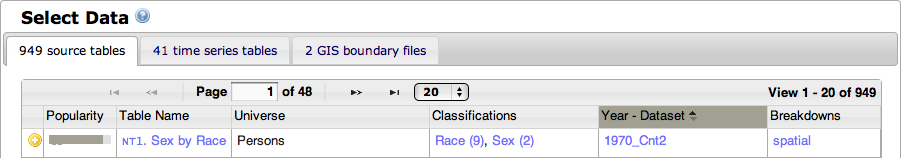
- A new dialog will appear, displaying a list of the various tables of information available for this topic and at this level of geography:
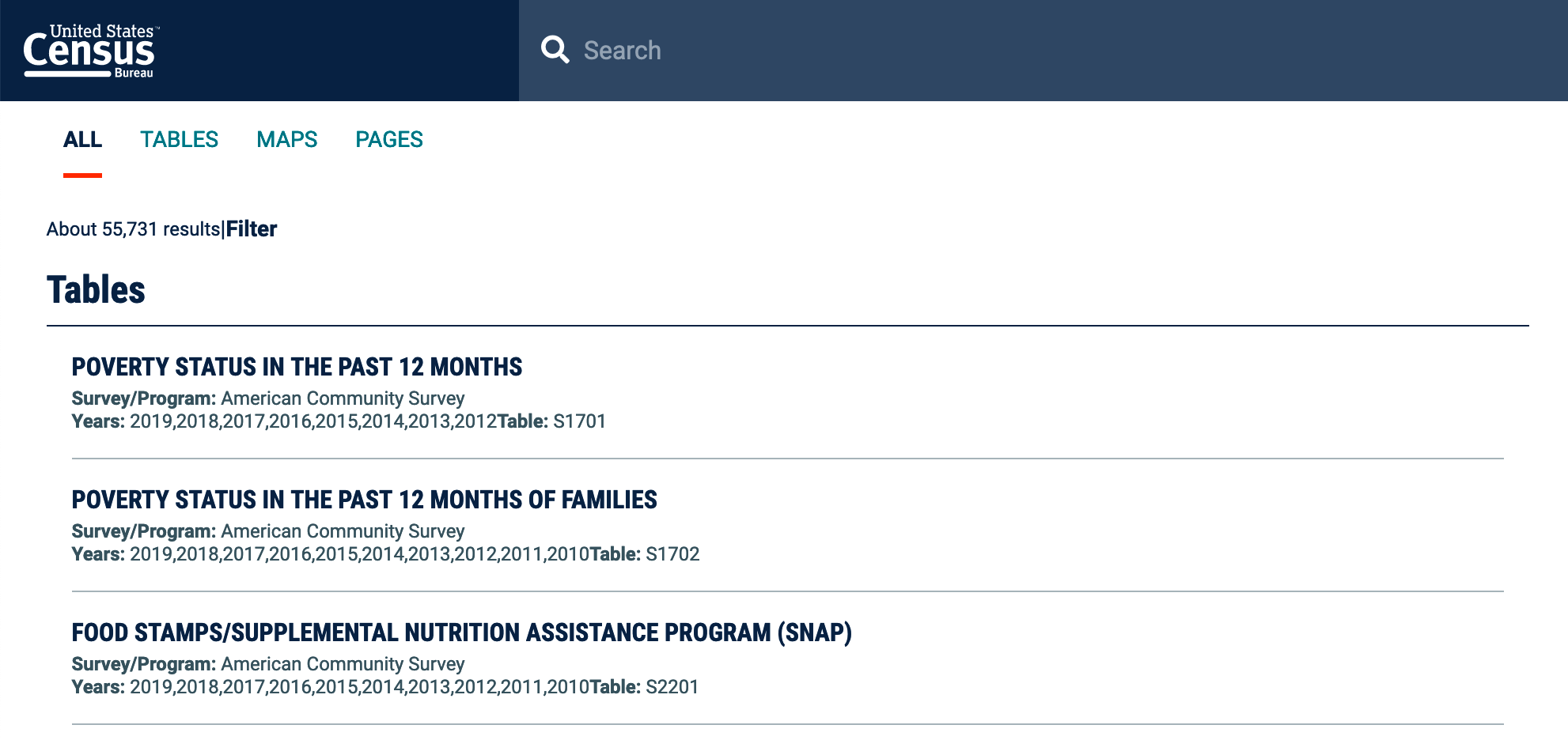
- In the list Tables,
click on, for example, POVERTY STATUS IN THE PAST 12 MONTHS, which expands to provide data on the poverty status of individuals in different categories:
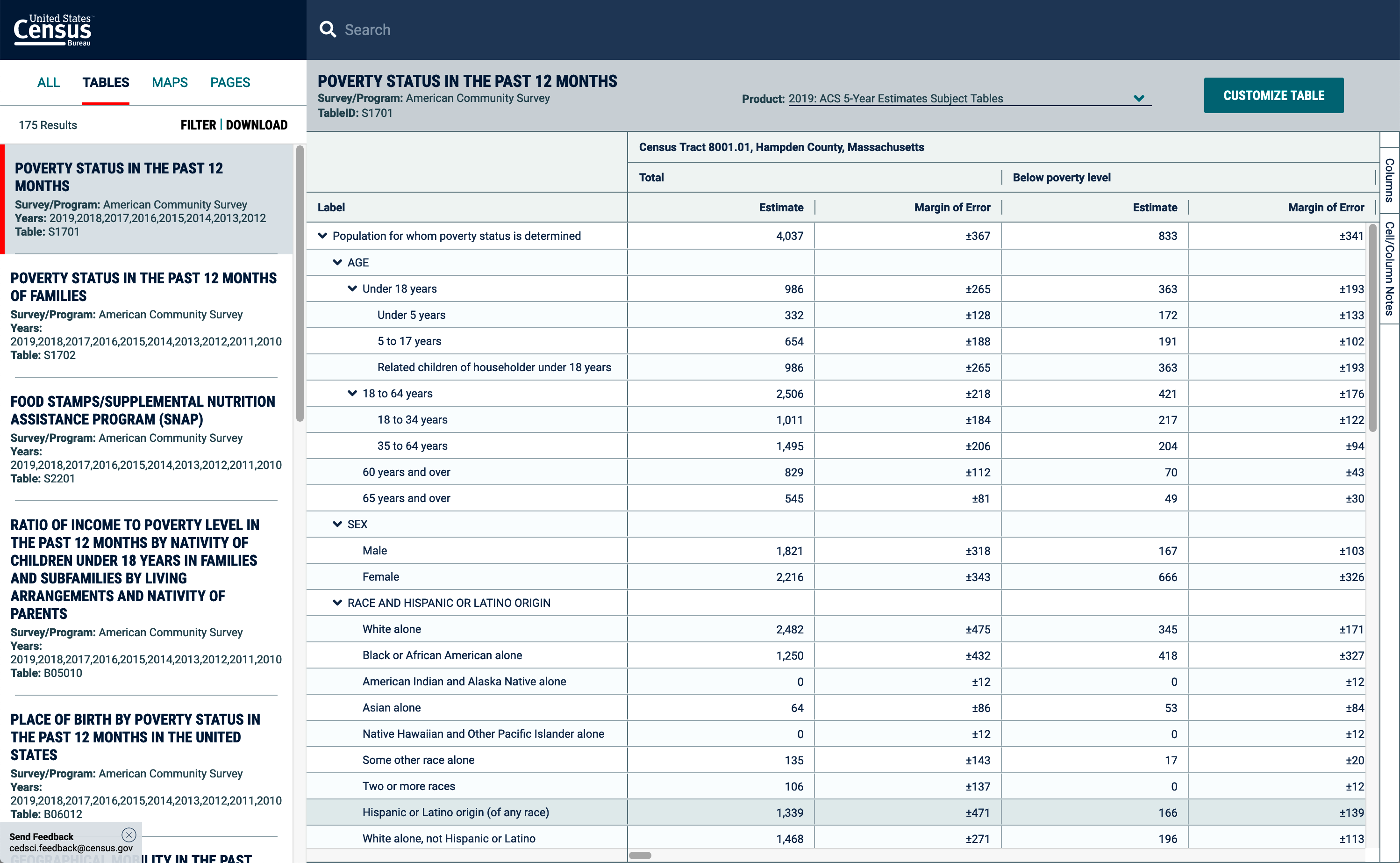
- At the top of the page, the menu Product shows the year and survey providing this particular set of data, e.g. 2019: ACS 5-Year Estimates Subject Tables.
With five years of data there are enough samples to provide useful information for this geographic type (tract), but with a margin of error on the order of 10%.
At the top of the page, clicking on the button
FILTER would open the dialog that allows you to change the geography type to a much larger one, e.g. County, which would let you see a more up-to-date table, the 1-year estimates, which would also have enough samples to reduce the margin of error to roughly 5%. (In general you could also select a smaller geography type, but it won’t actually let you see that data in this case because the margin of error would be significantly larger.) Click again on the button
FILTER to hide this dialog.
You can now review the data and scroll through it to make sure it has the information in which you’re interested,
e.g. the attribute Below poverty level for all individuals.
Here you can see the data that’s available for this combination of parameters: scroll down to see different subsets of the Population for whom poverty status is determined (breakdowns by age, gender, and race), and scroll to the right to see the different tracts and their number of individuals total and living in poverty. Note the subheadings of Estimate and Margin of Error.
You can also click on the different tables in the list on the left side to see their content.
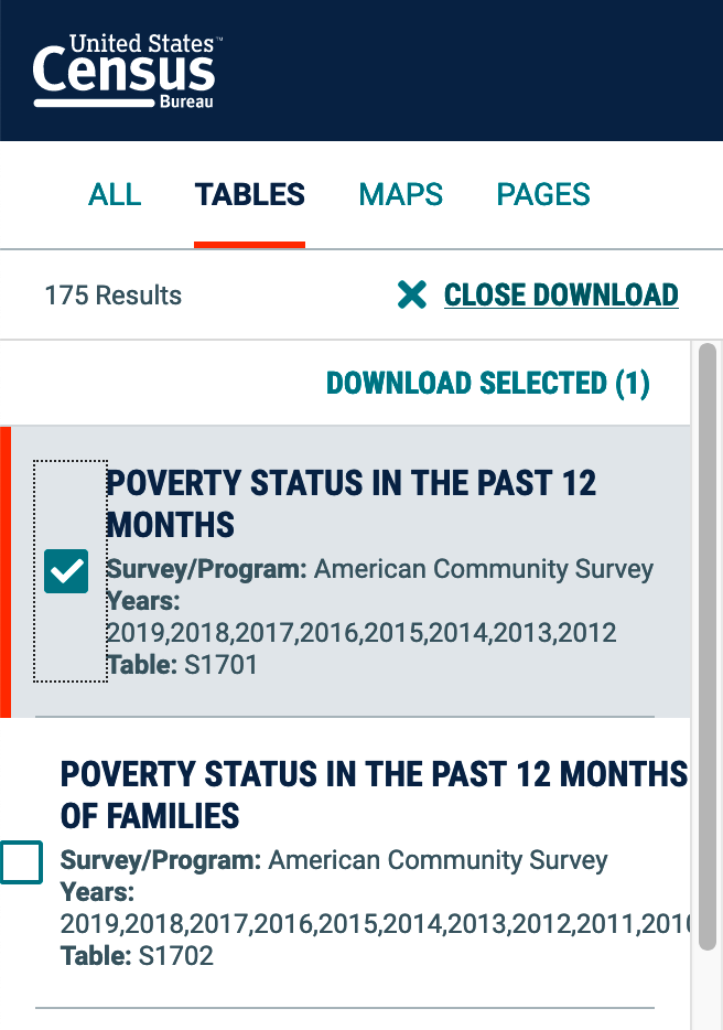 At the top of the page, click on the button DOWNLOAD. At the top of the page, click on the button DOWNLOAD.- The list of tables now reveals checkboxes next to them; click on the box next to the desired table(s), e.g. POVERTY STATUS IN THE PAST 12 MONTHS.
- Click the button DOWNLOAD SELECTED (#).
- In the dialog Download / Print / Share, note that one survey is selected, but you could add others if you wanted; and the default file type is CSV, which is correct for GIS. Click on the button DOWNLOAD.
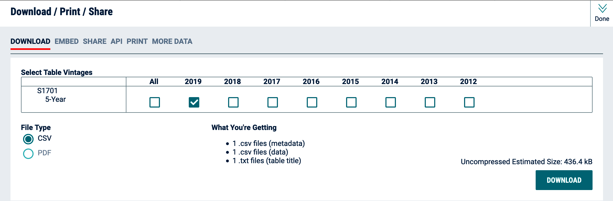
- In the next dialog We’re preparing your files, wait for the appearance of the button DOWNLOAD NOW, and then click it.
- The data will
be downloaded as a single compressed
file named something like
 ACSST5Y2019.S1701.zip. ArcGIS cannot see inside zipped files, so: ACSST5Y2019.S1701.zip. ArcGIS cannot see inside zipped files, so:
- Locate this file in your downloads folder, right-click on it to bring up its contextual menu, and select the menu item Extract All… ;
- In the dialog Extract Compressed (Zipped) Folders:
- Click on the button Browse…;
- In the dialog Select a destination, navigate to your folder MappingPlaceName;
- Click on the button New folder and give it a relevant name, e.g. ACSST5Y2019.S1701 or simply Poverty;
- Click on the button Select Folder.
- Now back in the previous dialog, click on the button Extract.
- The decompressed folder contains three files, with names like:
- ACSST5Y2019.S1701_data_with_overlays.csv — the actual census data, structured differently than above for use with GIS, with each tract in its own row.
- ACSST5Y2019.S1701_metadata.csv — a list of the various fields in the previous file providing explanations of what they represent. Such ”data about data” is known as metadata.
- ACSST5Y2019.S1701_table_title.txt — additional metadata providing background information such as source, methdology, etc.
You may have noticed in this last procedure
that the Census Bureau only has data online
starting in 2000. If you want data and boundary
files from earlier years, visit the National
Historical Geographic Information System,
which provides a similar system.
Once you’ve downloaded census data, you’ll need to clean it up to make it compatible with ArcGIS.
-
Double-click
on the file ACSST5Y2019.S1701_data_with_overlays.csv to
open it automatically in
 Excel and
inspect its contents: Excel and
inspect its contents:
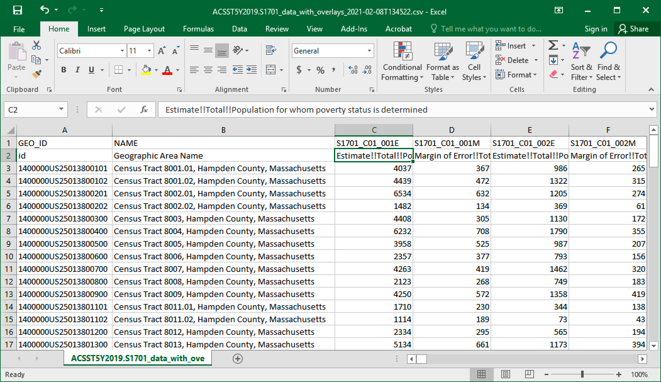
The first two rows have two versions of column headers, row 1 with short names, row 2 with longer, more descriptive names. The actual data begins in row 3.
The selected cell C2 has its content displayed in full in the formula bar above columns B and C: it’s the estimate of the total population for whom poverty status is determined (which is a subset of all survey respondents).
To easily see these descriptions, you have to either make the columns wider or make the rows higher and let the text wrap. For the latter:
- Select row 2 by clicking on the row header (i.e. the numbered box 2);
- Right-click on any one of them, and in the contextual menu that appears select
 Format Cells…; Format Cells…;
- In the dialog Format Cells, click the tab Alignment (if necessary), and in the area Text control check on Wrap text;
- Click the button OK and the row heights should increase to display their contents;
- Adjust the row heights and column widths to the desired amount by clicking and dragging the bottom and right borders of their headers, respectively.
- The descriptive labels in the second
row of a Census Excel file are important
for understanding the meaning of
the attributes. However, they are
too complex to be used as column
headers by ArcGIS — these names cannot include spaces, exclamation points, hyphens, etc.; they must include only letters (specifically the first character), numbers, and the underscore _ . So we will use
the first row instead.
Because column
headers must be immediately above the
data, we will swap the first two
rows:
- In the application Excel,
right-click on the row header 1,
just to the left of the column
header
GEO_ID, and in its contextual menu click on the menu item  Cut. Cut.
- Right-click on
the row header 3, and in its contextual menu click on the menu item Insert Cut Cells.
The cut row will be inserted before row 3, and the column header
GEO_ID into
the cell A2.
- Because we are
retaining the descriptive labels
in the worksheet, there will be non-table
data present in this worksheet. We must therefore name the
region of cells covered by the table,
and use that name when joining, instead
of the worksheet name (here called ACSST5Y2019.S1701_data_with_ove).
- Click on the cell in
the first row and first column
of the table, here the cell A2 containing
the column header
GEO_ID.
- Select the
entire first row of data by simultaneously holding down the keys Control and Shift and then pressing the key → (right arrow). The combination Control → by itself jumps to the end of the first contiguous block of data, while the combination Shift → adds just one cell to the original selection of the cell A2.
- Now add all of the other rows to your selection by again simultaneously holding down the keys Control and Shift and then pressing the key ↓ (down arrow).
- Click in the Name
Box
 that’s located
above column A,
which should contain the first cell name, A2, type a descriptive name,
e.g. Poverty,
and press the key Enter.
Note that spaces
and most special characters
aren’t allowed in these names. that’s located
above column A,
which should contain the first cell name, A2, type a descriptive name,
e.g. Poverty,
and press the key Enter.
Note that spaces
and most special characters
aren’t allowed in these names.
Named regions are known everywhere inside a workbook,
including within other worksheets.
The Name
Box has a menu button at its right end that lets you select any named regions you’ve defined. Names can also be defined, edited, and deleted by
selecting the menu Formulas
, looking in the section Defined Names, and then clicking on the menu item Name Manager.
- Modifications such as cell wrapping and named regions are not saved with CSV files, so this file should instead be saved as an Excelworkbook (this will also prevent annoying messages about loss of features whenever you save it in the original format).
- Select the menu File,
and then click on the list item Save As, and then click on the name of the current folder.
- In the dialog Save As, in the menu Save as type:, select Excel Workbook (*.xlsx).
- Click the button Save.
- Quit Excel, which will allow you to add this table to ArcMap.
Sometimes there’s no exact match between the fields in two tables, and a new one must be created:
When you want to join a source table to a target geography layer’s attribute table, the first step is to determine which fields, if any, match. Which columns have the same data or almost the same data? They may have different names, e.g. GEO_ID and GEOID10 in the previous procedure, but that’s actually not important as fields will be referenced individually when setting up the join. They may have differences in representation, e.g. abbreviations in one and full names in the other. There may be small differences or there may be large ones, but in either case you must make sure there are identical matches for every feature that you want to join.
Often you’ll need to create a new field and calculate a set of matching values. This can be done in either table, depending on their usage. If the attribute table is the best location for this new field, the Field Calculator in ArcGIS can be used to make small changes or automate this process for all fields when you can identify a simple pattern to the differences.
For example, in the previous procedure Making a Census File Compatible with ArcGIS Using Excel, compare the Excel table with the attribute table of MASSCENSUS2010TRACTS. The FIPS numbers in the latter show up in the former, but with an extra unvarying string prepended to it, 1400000US, which describes the type of data represented:
- The first three digits identify the summary level of the data;
140 means “State-County-Census Tract”.
- The next four digits are the “geographic variant” and “geographic component”, which in most cases are just set to
00 and 00.
- The last two digits provides an internationalization by using the International Standards Organization’s two-character country code, here
US for the United States of America.
 Since this geographic identifier will appear in all data downloaded from the Census Bureau, while the geography layer could be re-used many times, it’s better in this case to add a field to the latter and calculate matching values for the identifier: Since this geographic identifier will appear in all data downloaded from the Census Bureau, while the geography layer could be re-used many times, it’s better in this case to add a field to the latter and calculate matching values for the identifier:
- In the attribute table, click on the menu
 Table Options, and select the menu item Add Field…. Table Options, and select the menu item Add Field….
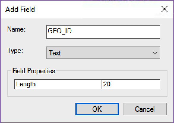
- In the dialog Add Field, in the text field Name, provide a name, e.g. GEO_ID.
- In the menu Type, select Text.
- In the section Field Properties, in the text field Length, provide a number — e.g. 20.
- Click the button OK.
 Before calculating values for a field, always check to make sure that no records are selected, or those will be the only ones to which the calculation will apply: in the table’s menu bar, if the button Before calculating values for a field, always check to make sure that no records are selected, or those will be the only ones to which the calculation will apply: in the table’s menu bar, if the button  Clear Selection is not grayed out, click on it. Clear Selection is not grayed out, click on it.- Locate the new field (usually the very last column), right-click on its header to bring up its contextual menu, and click on the item
 Field Calculator. Field Calculator.
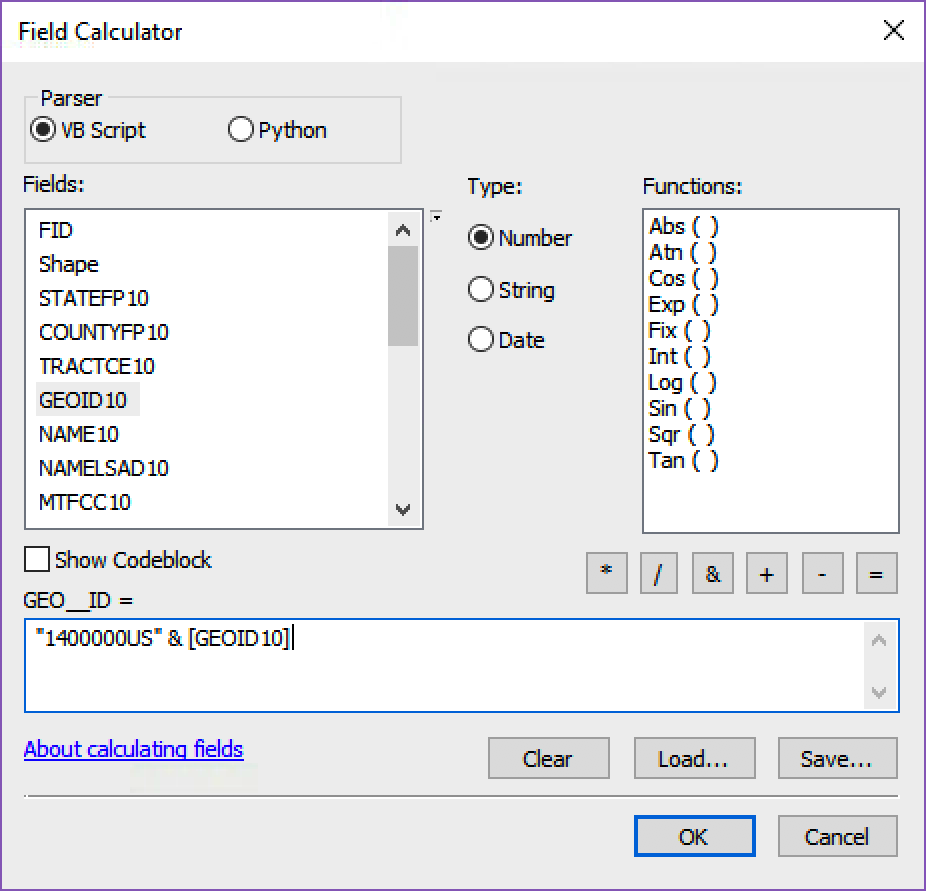
- In the dialog Field Calculator, in the text field field_name =, type an expression to update field values, e.g. to prepend the census identifier’s common text string to the FIPS value for that record:
"1400000US" & [GEOID10]
The VBScript language is used here by default, but Python could also be used (and often provides better tools for complex calculations). The text string must be surrounded by double quotes, and the field name used to provide this record’s value must be surrounded by square brackets; the & character is used to concatenate the two together. As an alternative to typing in the field name, you can also insert it by double-clicking on it in the list Fields:.
- Click the button OK, and the field should be populated with the correct values.
If you just need to change one field (e.g. state names but “District of Columbia” appears in one and “Columbia” in the other), you can select that one record, skip step 6 above, and run the Field Calculator with the matching value, and it will only change that one record.
To see the results of the previous two procedures, try out the new attributes:
- Follow this procedure and join the census
table ACSST5Y2019.S1701_data_with_overlays.xlsx to
the layer MASSCENSUS2010TRACTS using
the field
GEO_ID in both cases.
- Symbolize
the layer with one of
the quantitative fields from
the second layer, e.g.
S1701_C01_002E (Population
for whom poverty status is
determined: Below poverty level), normalized
by S1701_C01_001E (Population
for whom poverty status is
determined: Total).
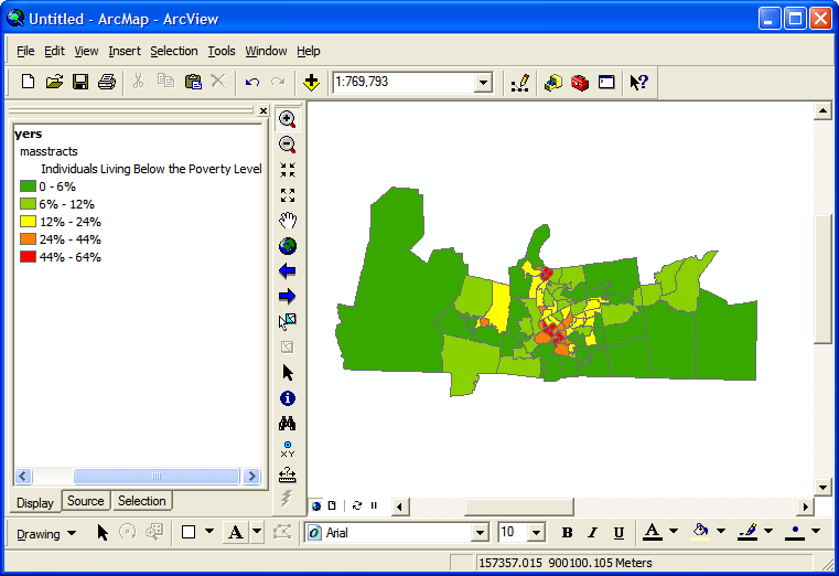
The areas in red above are in eastern Holyoke (the area known as “The Flats”) and in west-central Springfield, surrounding the downtown area.
Exercise: Mapping More Census Data
Revisit the Census Bureau’s data site as described in the procedure Downloading Census Data from the U.S. Census Bureau, find another topic of interest to you, e.g. educational attainment, download its data, and map it.
Do you have any ideas about how you might display both it and the previous poverty data on the same map?
While joining tables may appear
straightforward, they need to be in a certain
format to ensure success.
Before joining two tables using a particular
attribute, it’s generally a good idea to
ascertain the data type of that
attribute in the layer’s table. The reason
is that not only the join attribute’s values
but also its type must be compatible
in the two tables, and appearances can be
deceiving.
For example, the POP2010 number
in the attribute table for MASSCENSUS2010TRACTS may
appear to be an integer but it could actually
be text or a real number.
The following table describes the most common
data types.
Some Common ArcGIS Attribute Data Types
| Data Type |
Value Represented |
Minimum Value |
Maximum Value |
Maximum Significant
Digits/Characters |
| Short |
Integer number |
-32,768 |
32,767 |
5 |
| Long |
Integer number |
-2,147,483,648 |
2,147,483,647 |
10 |
| Float |
Real number |
-3.4
x 1038 |
1.2
x 1038 |
6 |
| Double |
Real number |
-2.2
x 10308 |
1.8
x 10308 |
15 |
| Text |
String of characters |
— |
— |
254 |
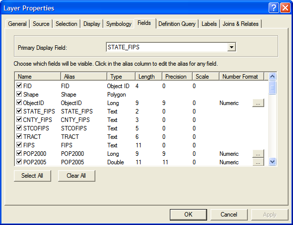
We can see in the image above that the data
type of the FIPS attribute in MASSCENSUS2010TRACTS is Text.
Question: Could
it be another type?
To use this attribute to join an Excel table,
the corresponding attribute data type must
also be Text. If you look
at this Excel
table and the join field we used, GEO_ID2,
you’ll note the little green flag in the
upper left corner of each cell; it indicates
that the numbers are actually formatted as
text. (Hint: this can also be ascertained
from their alignment on the left; Excel aligns
numbers on the right.)
Another formatting incompatibility to be aware
of is that the content of a cell in the Excel
join column cannot wrap, i.e. it
must all be on one line, and cells in the
table shouldn’t be merged cells,
either.
More generally, the data in the two join columns
must match exactly. In particular,
watch out for extra spaces between words
and at the beginning and end of data.
Summary: Making an Excel File Compatible
with ArcGIS
While Microsoft Excel can make it easy to
manipulate data tables, it also has its own
way of doing things with which you’ll need
to be familiar to make extensive use of it.
Such use is outside of the scope of this
class, but if you follow the recommendations
below, your data tables should be compatible
with ArcGIS.
Generally speaking there are five things
you need to do to make Excel data compatible
with ArcGIS: name it properly, create
a row of field names, below that arrange
your data in a plain rectangular array,
name the table, and make sure the join
fields match. Below are general descriptions
of how to do this.
- Name the file:
it should start
with a letter and afterwards include only letters,
numbers, and underscores.
- Create a row of field names:
- The very
first row in a table must contain
unique names for each column.
Usually they will in some way
describe the attribute that will
be in that field, e.g. Population,
ZipCode, etc.
- Field names must begin with letters,
and after that can contain letters,
numbers, or the underscore _
. They cannot contain other special
characters such as the period
. or hyphen -,
or spaces (and be careful that
you don’t have any spaces at
the beginning or end of the names,
too!). Note that
field names are also case
sensitive (upper
and lower case letters are distinguished).
If your joined data appears
as <null>, then check the
field names for an illegal
character.
- Field names
cannot be one of a long list
of reserved
words, e.g. All. If
your joined data appears
as <null>, then check the field
names against this list.
- For some types of joined tables,
field names must be ten characters
or less, though in other types you
can use up to 64 characters.
It’s a good idea to use short
names in any case.
- Arrange your
data in a plain rectangular array:
- Every map feature, such as a
state or city, must have its
data in a single row.
- Every column/field
should contain the same kind
of information for each feature,
e.g. all population values should
be in a single column. Blanks
are allowed if particular data
is missing. Also make sure the
values have a consistent data
type, e.g. all text, all integers,
or all real numbers.
- All record and feature data must
be contiguous, i.e. there must
be no other data or blank rows
or columns separating the data,
and it must begin immediately below
the field name row.
- Name the table:
- If you have non-table data in
the cells around your table,
e.g. explanatory notes, you’ll
want to select just the range
of cells covered by the table
and give it a unique name.
- If you don’t
have any other data in the worksheet
besides your table, and it begins
in cell A1, then the table can
be referenced by its worksheet
name. It’s highly recommended
that you change the worksheet
name to something more illuminating
than
Sheet0. Whatever
name it has, ArcGIS will see
it with a $ at the end, e.g. Sheet0$,
indicating that it’s using the
entire contents of the worksheet.
- Unlike field names, worksheet
and cell range names have few
restrictions like those described
in (1)(b) above. However, names
with spaces and special characters
in them will appear with single
quotes around them, e.g. 'My
Sheet$'.
- Make sure the
join fields match:
- Make sure the data types in the
join fields are compatible: both
text, both integers, or both
real numbers.
- Make sure
the Excel join field doesn’t
wrap its text and doesn’t have
any merged cells.
- Make sure the values in the two
join fields match exactly, e.g.
there are no extra spaces, variations
in case, etc.
- The two tables
don’t need to have the same number
of records, e.g. some features
could be missing in one table
or the other. If the map layer
is missing a record that appears
in the join table, the latter
will be ignored, and if the join
table is missing a record that
appears in the map layer, its
values will appear as
<Null>.
Street addresses can be geographically
located when you have a special street layer
and a geocoder.
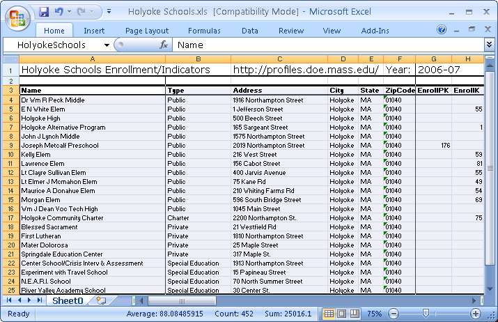
Geographic data often comes in the form of
a table of street addresses, for example
of schools or businesses, along with attributes
describing them such as their name, purpose,
etc.:
 A
full street address includes a street number,
street name, city, state, and zip code. Like
other place name data, street names
can be associated with a street layer to
get a very rough location. To get a more
accurate position, we need to know where
the street numbers fall along the street. A
full street address includes a street number,
street name, city, state, and zip code. Like
other place name data, street names
can be associated with a street layer to
get a very rough location. To get a more
accurate position, we need to know where
the street numbers fall along the street.
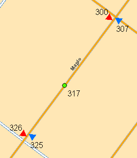
If a street layer contains details about which
addresses lie within which blocks, it can
be used with a program called a geocoder to
place the addresses on the map as points
along the streets. Address locations will
be approximate, because only a block’s beginning
and ending addresses are usually provided,
and others are linearly interpolated along
the street (see the block at the right, which
places the address 317). In addition, street
layers have varying degrees of accuracy.
Street layers are commonly available from
cities and towns as well as commercial entities.
The ArcGIS software suite comes with the
collection ESRI Data and Maps,
which includes the commercial package called Street
Atlas North America, and a geocoder that works
with it.
- In ArcMap,
in the toolbar Standard,
click on the button Add
Data.
- In the dialog Add
Data, make a new connection
to the folder K:\Maps (see Constructing
and Sharing Maps for details).
This network folder is where
Amherst College stores a large
amount of data for use in maps.
- Navigate into the folder ArcGIS Books-n-Data\ESRI Data & Maps 2013\streetmap_na.
- Click on the
file
 StreetMap North
America.lyr.
This is a layer file,
which references data in one or more
additional files, along with information
about how to symbolize them. StreetMap North
America.lyr.
This is a layer file,
which references data in one or more
additional files, along with information
about how to symbolize them.
- Click on the button Add.
- You will now see the dialog Geographic
Coordinate System Warning;
you don’t have to worry about
this for now, so click on the
button Close.
- Click on the
button
 Zoom In,
and click-and-drag a rectangle around
the City of Holyoke (north of Springfield
and I-90, east of I-91). Zoom In,
and click-and-drag a rectangle around
the City of Holyoke (north of Springfield
and I-90, east of I-91).
- In the Table of Contents,
turn off and back on the layer StreetMap North
America by
clicking on the checkbox to
the left of its name, and notice
the relationship of the two data
sets.
Let’s now geocode a set of addresses using
Street Atlas’ street information:
- In ArcMap,
click on the menu Tools,
then select the submenu Geocoding,
followed by the menu item
 Geocode Addresses…. Geocode Addresses….
- The dialog
 Choose an Address Locator to use… will
appear with a list of address
locator databases. If this is
first time you’ve geocoded this
list will be empty, and you’ll
need to choose the correct encoder
for the street address database
format: Choose an Address Locator to use… will
appear with a list of address
locator databases. If this is
first time you’ve geocoded this
list will be empty, and you’ll
need to choose the correct encoder
for the street address database
format:
- Click on the
button Add….
 In
the dialog Add Address Locator,
navigate into the folder K:\Maps\ArcGIS Books-n-Data\ESRI Data & Maps 2013\streetmap_na\data. In
the dialog Add Address Locator,
navigate into the folder K:\Maps\ArcGIS Books-n-Data\ESRI Data & Maps 2013\streetmap_na\data.- Double-click
on the file Street_Addresses_US.
- Continuing
in the
dialog Choose an Address Locator to use…,
click
on the button OK.
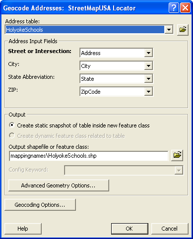
- In the dialog Geocode Addresses: Street_Addresses_US,
the menu Address table: might
already list your data set if
you’ve previously added it. Otherwise:
- Click on the button Browse and
navigate into the folder
with the table to be joined,
e.g. MappingPlaceNames.
- Double-click
on the table to be joined,
e.g the Excel workbook Holyoke Schools.xls.
- In the workbook, double-click
on a sheet or a named region,
e.g. HolyokeSchools.
- Continuing in the dialog Geocode Addresses: Street_Addresses_US,
verify that
the Address Input Fields match
the correct ones in your data
table.
- Make sure the Output
shapefile or feature class: is
an appropriately named and
located file, e.g. HolyokeSchools.shp in
the folder MappingPlaceNames.
- Click on
the button OK.
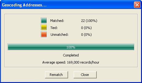 The
dialog Geocoding Addresses… will
now appear and provide a summary
of the geocoding. It will tell
you how many of the addresses
in the table were matched, tied,
or unmatched (e.g. if a zip code
is incorrect it may end up tied
with a slightly different street
name). The
dialog Geocoding Addresses… will
now appear and provide a summary
of the geocoding. It will tell
you how many of the addresses
in the table were matched, tied,
or unmatched (e.g. if a zip code
is incorrect it may end up tied
with a slightly different street
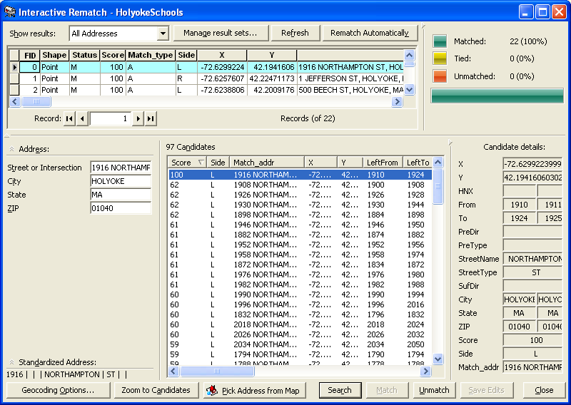
name).- If you have not matched all of
the records (very common),
you may want to look at how the
matches are made. Click on the
button Rematch;
the dialog Interactive Rematch will
appear. It lists each
record and gives it a
score from 0 - 100 judging
the quality of the match.
You can use this dialog
to interactively improve
the match, e.g. by
correcting bad data or
choosing a more likely
address (N.B. sometimes the geocode
database can be wrong,
too!).
This dialog can be recalled later by clicking on
the menu Tools,
then selecting the submenus Geocoding and Review/Rematch Addresses,
and finally clicking
on the menu item Geocoding Result: ….
- When you are finished matching,
click on the button Close.
- The resulting
data will be added to the
map with a distinguishing name,
e.g. Geocoding Result: HolyokeSchools.
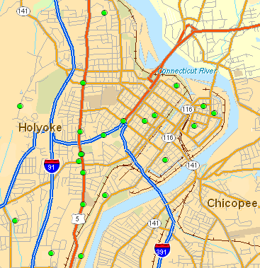
Note that these points on the map are
created relative to Street Atlas’ description
of the streets; this may differ from
other descriptions, e.g. the local Planning
Department may have more accurate data,
while an old map may be less accurate.
|