Geographic
data is commonly in the form of raster
images, such as scanned maps, aerial or satellite photos, and
elevation grids.
Geographic raster
images have some basic features but still come
in a wide variety of formats, which are used
for specific purposes.
The Spatial Location of Raster Data
Recall that raster data, such as orthophotos or scanned maps or elevation
models, consist of a grid of pixels
whose values say something about the surface
of the Earth:

Like vector data, the raster data used by GIS will always be defined
in one particular spatial reference, where it
is a rectangular grid.
However, raster data must also
provide the following information relative to
the coordinate system of the spatial reference:
- The location of one pixel (e.g.
the center of the upper-left pixel);
- The size of its pixels, e.g. meters or
degrees, which will be either
square (usually) or rectangular (rarely);
- The amount of rotation of the raster relative to the easting
and northing directions.
This transformation information allows the position of
every pixel to be calculated and correctly displayed
relative to other data, and such rasters are
said to be georeferenced.
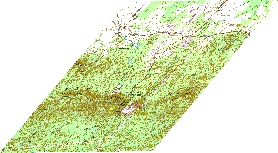
Not surprisingly, when a raster is reprojected to another spatial
reference, it will appear with a distorted shape:
|
|
Massachusetts State
Plane |
Sinusoidal |
The transformation information is stored in a number of
ways, such as a separate world
file, commonly
provided on the Internet for georeferenced rasters,
e.g. .tfw.
Unfortunately
the world file format does not also include the
spatial reference, so you must look for that
information separately, as an associated .prj
file
or as a textual description that you must incorporate
in the
same way as for vector data.
Both types of information will be stored in a .aux file.
The Representation of Pixel Data
Pixel data can be expressed in
a number of different formats. Some of the more
common ones are:
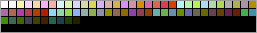
 Color
Map or Indexed
Color: A single value that is
an index into a palette of colors stored
with the raster: Color
Map or Indexed
Color: A single value that is
an index into a palette of colors stored
with the raster:
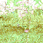
Besides limited-color
printed materials, such as the scanned
map to the right, these values may also represent
categorical data such as soil type, etc.
 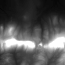 Grayscale:
A single value that is commonly displayed
using a ramp ranging
between black and white Grayscale:
A single value that is commonly displayed
using a ramp ranging
between black and white  Such
a ramp is used for "black-and-white" photographs
as well as other data. Such
a ramp is used for "black-and-white" photographs
as well as other data.
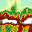
Non-photographic data could also be displayed
with another color ramp such as
 ,
which is commonly used for elevation. ,
which is commonly used for elevation.
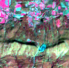 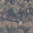 RGB:
A triplet of values that is displayed on
your computer screen as a visually merged
color: RGB:
A triplet of values that is displayed on
your computer screen as a visually merged
color:
This
format is used for color photographs, along
with satellite imagery that may substitute
another wavelength of light such
as infrared, known as Color-Infrared (CIR).
The number of values assigned to each pixel is referred to as
the number of bands or channels. Multispectral
satellite imagery can have seven or more bands
per pixel, but computer display technology will
show at most three of them at once.
The values used for each pixel band may be one of several numeric
types:
Raster Pixel Types
| Pixel Type |
Pixel Depth |
Minimum Value |
Maximum Value |
| Unsigned Integer |
8 bit = 1 byte |
0 |
255 |
| |
16 bit = 2 bytes |
0 |
65535 |
| |
32 bit = 4 bytes |
0 |
4294967295 |
| Signed Integer |
8 bit = 1 byte |
-128 |
127 |
| |
16 bit = 2 bytes |
-32,768 |
32,767 |
| |
32 bit = 4 bytes |
-2,147,483,648 |
2,147,483,647 |
| Floating Point (Real) |
32 bit = 4 bytes |
-3.4
x 1038 |
1.2
x 1038 |
| Double Precision (Real) |
64 bit = 8 bytes |
-2.2
x 10308 |
1.8
x 10308 |
Generally speaking, the greater the depth, the larger the file
size of the raster, so smaller depths are used
when possible.
For example, if you have an elevation range that varies between sea
level (0 m) and 200 m, and you don't need fractional
values, you could use one-byte unsigned
integers.
If you have a color photograph, the three RGB channels will need
at least three integer bytes; but because of
the power-of-two design of computer architectures,
they are commonly stored as a four-byte quantity.
The fourth byte will sometimes hold information about a pixel's degree
of
transparency (or its inverse, opacity); it is
then known as an alpha channel.
For most imagery formats ArcGIS can view the individual color channels.
When opening such images, ArcMap and ArcCatalog
treat them as “folders” that open up to list
Band_1, Band_2, …. So if you want to
view the combined format, you can’t double-click
on the file, you need to click on it
once and then click the button Add.
Often a rectangular raster will include pixels that cover locations
that can't be assigned actual values, e.g. in
an elevation data set that might lie over water.
Such pixels are typically assigned a value or
value combination that is understood to represent NoData.
If ArcGIS can determine what that "color" is, it will display
it as completely transparent (this special value
may be stored in an associated .aux file).
Rasters may be stored in a number of different
formats, which may or may not be compressed to save
space. The greatest compression is usually achieved
by using a lossy
compression format that will
not perfectly reconstruct the original data.
Raster File Formats
| File Format |
File
Extension |
World File
Extension |
Pixel Type(s) |
Compression |
Description |
| Windows BitMaP |
.bmp |
.bpw, .aux |
Colormap
Grayscale
RGB |
None (usually) |
The standard Windows image
format, very basic. |
| Graphics Interchange Format |
.gif |
.gfw, .aux |
Colormap |
Lossless |
A compressed image format
that is commonly used on the Internet
for images with simple colors and structures,
e.g. line drawings and simple scanned maps. |
| Portable Network Graphics |
.png |
.pgw, .aux |
Colormap
Grayscale
RGB |
Lossless |
A compressed image format
that is replacing .gif on
the Internet due to its better compression
and more flexible pixel types. |
| Tagged Image File Format |
.tif, .tiff |
internal
.tfw,
.aux |
Colormap
Grayscale
RGB |
Optional lossless |
Commonly
used for photographic
work as well as scientific imaging,
its use on the Internet is uneven due
to its many variations.
A new version of the format, GeoTIFF,
embeds transformation information in
the TIFF header. |
| Joint Photographic Experts
Group |
.jpg, .jpeg |
.jpw, .aux |
Grayscale
RGB |
Lossy (can be lossless) |
An
open standard that is commonly
used on the Internet for photographs
and other images with many gradations
of color. |
| Joint Photographic Experts
Group 2000 |
.jp2 |
.j2w, .aux |
Grayscale
RGB |
Lossy (can be lossless) |
A newer open standard
that
stores multiple resolutions (scales).
It is not yet completely supported on
the Internet. |
| Multiresolution Seamless
Image Database |
.sid |
internal
.sdw
.aux |
Grayscale
RGB |
Lossy (can be lossless) |
A proprietary format that
stores multiple resolutions (scales).
Supported on the Internet only via web
browser plug-in. |
| GRID |
None |
.aux |
Grayscale
RGB |
Lossless |
ESRI's proprietary image
format, not supported
on the Internet. |
The .aux format is ArcGIS-specific, so it will
be less common even though it's more convenient,
including both transformation and projection
information. If present it will take precedence
over a world file.
In addition to the auxiliary files, another associated
ArcGIS file you may come across is the pyramid file,
with file extension .rrd. It holds lower-resolution
versions of the original image to facilitate
rapid display when it's viewed at smaller
scales. Multi-resolution files such as JPEG2
and MrSID include pyramids as part of
their definition. When you add other formats
lacking a pyramid file to a map, ArcGIS will
ask if you want to build one; generally
this is a good idea.
ArcGIS also stores statistics information for
images in .xml files.
Rasters are far more prevalent
on the Internet than other formats such as shapefiles
or even XY tables, because they are often
images that can be directly viewed. Make sure
to also download associated world files, projection
files, et al.!
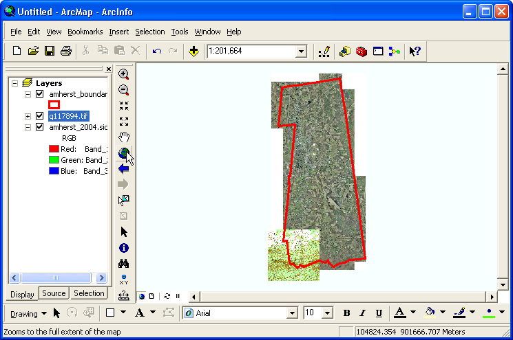
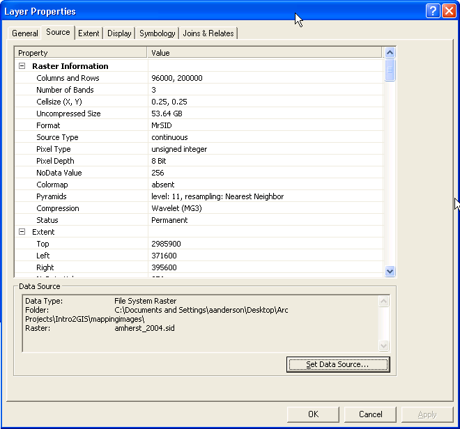
- In
 ArcMap,
in the Table of Contents,
double-click on the raster of interest,
e.g. ArcMap,
in the Table of Contents,
double-click on the raster of interest,
e.g.  amherst_2004.sid or q117894.tif. amherst_2004.sid or q117894.tif.
- In the dialog Layer Properties,
click on the tab Source.
- Read the table Property | Value:
- In the section Raster Information,
you should note the following:
- The number
of Columns and Rows in
the raster (in this example,
they are equal so it's
square)
- The Cellsize (X,
Y) (pixel size) in the
units of the coordinate
system (in this example,
it's again square).
- The file Format;
- The Number of Bands per
pixel;
- The Pixel Type and Pixel Depth;
- If a Colormap is used;
- If a NoData value is assigned;
- If Compression is
used.
- Scrolling down to the section Spatial Reference,
you should note what that is,
and also its Linear Unit (if
it has one).
- Scrolling up to the section Extent,
note the distance the raster
covers in each direction
Exercise: How does
the other raster differ?
Traditional paper maps contain a great deal of geographic
information, so it's important to be able to
incorporate them into GIS.
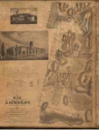
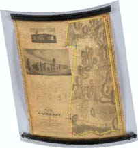
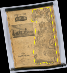
A
Map of Amherst with a View of the College
and Mount Pleasant Institution
by
Alonzo Gray & Charles
B. Adams,
Published May 1833 by
Pendletons
Lithography, Boston, MA.
(Source: The David Rumsey
Historical Map Collection, http://www.davidrumsey.com/).
Paper maps are ubiquitous,
and often they contain data that are useful
in a GIS map, e.g. as a background for other
data or to compare modern features with historical
locations.
A paper map must first
be scanned into a digital format, a now-common
procedure that
we won’t
go into here.
Scans of paper maps
and aerial photos must then be spatially positioned
to use them with other GIS data, a process
known as georeferencing.
To position the scanned map so that it aligns
with other GIS data, we can compare it with known
reference points or control points, e.g. from
an existing digital map or as collected by a
GPS receiver.
At a minimum a scanned
map must be moved to its correct geographic position,
oriented properly, and scaled to its correct
size; this requires at least two control points.
Sometimes
traditional maps are distorted; this might be
due to:
- Poor measurement;
- Intentional focus
on the relative position of features;
- Non-vertical perspective, e.g. in aerial
photos and panoramic
maps;
- Unknown projection.
Such distortions
will likely require a non-uniform scaling to
align with known features; this requires at least
six control points.
For this procedure you must already have a
scanned map available, e.g. the 1833 map
of Amherst shown above.
You must also have some reference
layers for comparison, such as boundary
files, orthophotos, or GPS points.
- Begin by adding the reference layer(s)
and scanned map to ArcMap:
- Add one or
more reference layers for
comparison, e.g.
 amherst_boundary.lyrand amherst_2004.sid (see Constructing
and Sharing Maps for
details). amherst_boundary.lyrand amherst_2004.sid (see Constructing
and Sharing Maps for
details).
- If you know or can guess
the projection of the scanned
map, change the spatial reference
of the map to match (see Mapping
Geographic Coordinate Data for
details). Otherwise, if you
don't want to match the
reference layer(s), a
good option is Mercator,
since it is shape-preserving
and also orients north upward,
a common characteristic of
paper maps.
- Add the scanned map, e.g. amherst1833.sid.
- In the dialog ArcMap,
you will be advised that One
or more layers is missing spatial
reference information…;
click on the button OK.
- Because the scanned map has
no spatial reference information,
it will be positioned at
the origin of coordinates,
typically far from the reference
layer(s).
- Optional
Step: In the toolbar Tools,
click on the button
 Full Extent.
Viewing the full extent of
the data will likely produce
two widely separated specks,
one the correctly positioned
reference layer(s) and the
other the unplaced scanned
map. Can you tell which is
which? Full Extent.
Viewing the full extent of
the data will likely produce
two widely separated specks,
one the correctly positioned
reference layer(s) and the
other the unplaced scanned
map. Can you tell which is
which?
- To view the scanned map,
right-click on its name
in the Table of Contents and
then click on the menu item
 Zoom To Layer. Zoom To Layer.
- Examine the added map and
get a good idea of its extent
and any marked boundaries.
- Return to the original location
by right-clicking on a reference
layer's name
in the Table of Contents and
then clicking on the menu
item Zoom To Layer.
- Z
 oom in or out from the reference
layer so that its recognizable
features roughly match those
of the scanned map. oom in or out from the reference
layer so that its recognizable
features roughly match those
of the scanned map.
- Now initiate the georeferencing process:
- If
the Georeferencing Toolbar is not already
visible, click on the menu View,
then point at the menu item Toolbars,
then click on the menu item Georeferencing.
After the toolbar appears, you
can dock it out of the way, by
clicking-and-dragging it anywhere
around the window frames.
- In the toolbar Georeferencing,
click on the menu Layer:,
then click on the menu item for
the scanned map (if
isn’t already selected — ArcGIS
will list all
image layers without a spatial
reference, and more than likely
this will be the only one).
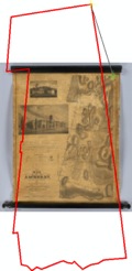
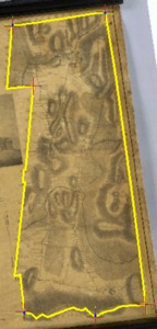
- Click on the menu Georeferencing,
and then click on the menu item Fit
to Display. The result
will look something like
the image at the right.
- This is a good time to save your
map; in the toolbar Standard,
click on the button
 Save. Save.
- You
must now add a control point that
links the same recognizable
location on the two layers, by first
clicking on it on the scanned map,
and second clicking on it on the reference
layer.
- Locations on the scanned map
are recognizable in a number
of ways:
- Point features are typically
labeled;
- Linear features such as streets,
railroads, rivers, canals,
and political boundaries
are usually labeled and have
intersections or sharp corners;
- Survey markers will often
have explicit coordinates
printed next to them;
- A graticule will
have intersections
of meridians and parallels
and explicit coordinates
at the map edges.
In the last two cases
it's usually easiest to guess
a coordinate location on
the reference map and then
correct
it later, as described below. Warning: to
use such coordinates
you must be working in the
spatial reference of the
scanned map!
- When you have identified
a location on both maps, in
the toolbar Tools,
click on the button
 Zoom In,
and then click and drag across
both layers to draw a rectangle
containing this location on
both maps. Zoom In,
and then click and drag across
both layers to draw a rectangle
containing this location on
both maps.
- If you can't clearly distinguish
this location on the scanned
map, drag another
small rectangle around it to
zoom in further.
- In the toolbar Georeferencing,
click on the button
 Add Control Points. Add Control Points.
 In
the scanned map, click on this
recognizable location. In
the scanned map, click on this
recognizable location.- If you’ve made a mistake,
you can hit the key Escape to
stop the link, and then continue
with Step (i).
- If you zoomed in a second time
in Step (b), then in the toolbar Tools
click on the button
 Go Back To Previous Extent. Go Back To Previous Extent.
- If you can't clearly distinguish
the recognizable location on
the reference layer:
- In the toolbar Tools,
click on the button Zoom In,
and drag another
small rectangle around
it to zoom in further.
- In
the toolbar Georeferencing,
click on the button Add Control Points.
Notice that it still
remembers that you
have already initiated
a control point by
clicking on the scanned
map.
 In
the reference layer, click on
the recognizable location. In
the reference layer, click on
the recognizable location.
The scanned map will
now shift its position to bring
the two points into alignment.- In the toolbar Tools,
click on the button Go Back To Previous Extent to
return to the overview.
- Repeat Step 3 with a second recognizable
location; this will uniformly scale
and rotate the map to align both
the first and second points.
- Repeat Step 3 a third time using a point that's
widely separated from
the line connecting the first two
points. This will nonuniformly scale
the map and rotate it to align all
three points. This is called a first-order
polynomial (affine) transformation.
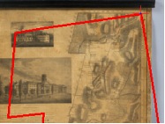
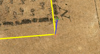 After
a fourth application of Step 3,
most likely the two points linking
the ends of the control point will no longer
be perfectly aligned, having some residual
distance represented
by a blue line, as seen to the left.
This is because there are no additional
free parameters in this transformation,
and a best
fit must
be calculated. After
a fourth application of Step 3,
most likely the two points linking
the ends of the control point will no longer
be perfectly aligned, having some residual
distance represented
by a blue line, as seen to the left.
This is because there are no additional
free parameters in this transformation,
and a best
fit must
be calculated.
- For most applications you will want
to repeat Step 3 several more times,
using points around the edge and
then throughout the middle of the
area of interest.
- A full description of the control
points you have set up is
provided in the Link
Table.
 In
the toolbar Georeferencing,
click on the button In
the toolbar Georeferencing,
click on the button  View Link Table. View Link Table.
The dialog Link Table should
now appear, listing each
control point link and their
starting (Source)
and ending (Map) locations.- If you click on any control point
link in the table, it will also
be highlighted in yellow on the
map.
- The link table
provides information about the
residual distance between between
the two ends of a control point
link, and the Total
RMS Error,
an average of the residuals,
which describes how far
out of alignment the entire
transformation is. We would
like it to be as small as
possible. Comparing individual
residual distances to the
total RMS error can indicate
which control points are
unusually separated. This
might be due to:
- poor surveying;
- rerouting of roads, railroads,
or canals, and the meandering
of rivers;
- deliberate abstractions,
e.g. the separation of features
to make them more distinguishable;
- bad GPS readings;
- accidental clicks.
These
points can be removed
from consideration by
clicking them in the
table and pressing the
key Delete.
- The X and Y values in the Link
Table are editable; this is most
useful if the control points
are survey markers or graticule intersections
whose values are printed on
the map, and can be typed into
the fields XMap and YMap.
- Warning: ArcMap
does not store information about
the link table, so to be able
to return to where you left off
after quitting or to restore
from a crash, you should periodically
save your table by clicking on
the button
Save… .
This will let you create a text
file storing your control points
that can be reloaded later by
clicking on the button
Load… .
- Click on the button OK
to dismiss the Link Table dialog.
 Another
way to improve the fit is to use nonlinear transformations. Their effect on the scanned
map may not always be desirable (for example,
you wouldn’t use them
on a presumably accurate map that
merely needs to be positioned). There are
several options available: Another
way to improve the fit is to use nonlinear transformations. Their effect on the scanned
map may not always be desirable (for example,
you wouldn’t use them
on a presumably accurate map that
merely needs to be positioned). There are
several options available:
- In
the toolbar Georeferencing,
click on the button View Link Table.
- In the dialog Link Table,
click on the menu Transformation:,
and then click on one of the following
menu items:
- If you have at least
six control
points, the item 2nd
Order Polynomial becomes available.
With exactly six, the Total
RMS Error will be
zero.
- If you have at least ten control points, an
additional option is 3rd
Order Polynomial . With exactly
ten, the Total RMS Error
will be zero.
- Also available with at least ten control points
is the option Spline.
It provides an exact
fit for all additional control
points, but can be very slow
due to the large number of
calculations required.
- An option available at all levels is Adjust;
it is very fast for even
hundreds of control points,
but produces discontinuities
in the image at the points'
exterior boundary.
- Click
on the button OK
to dismiss this dialog.
- Once you’re satisfied with the fit of the transformed
map, you can save it as a new raster
layer for later use. Be aware that this
process can take a while for a large
map.
- It's a good idea to first save your control
points as described in Step 8(c).
- In the dialog Georeferencing,
click on the menu item Rectify….
- In the dialog Save as,
in the text field Output
Location:, click on the
button
 Browse and
select the folder (not the file) where
you want to save the new raster. Browse and
select the folder (not the file) where
you want to save the new raster.
- In the menu Format:,
choose an output
format; for
scanned maps, JP2 or JPG is preferred,
though PNG can also be good for
relatively simple images. JPG
is the most compatible with external
applications and will typically
produce the smallest files if
you are willing to sacrifice
image quality.
- If you choose JP2 or JPG, in the text field Compression
Quality (1-100): type
a value or leave the
default (anything less
than 100 will be lossy).
- In the text field Name:,
adjust the file name to be more
descriptive, e.g. amherst1833rectified.jp2.
Don't change the file extension
here, use Step (d) instead. Warning:
GRID-format names must have a
base that's less than 13 characters
long.
- Click on the menu Resample
Type:, and then click on one of the
menu items Bilinear Interpolation or Cubic
Convolution(better but slower). The
option Nearest Neighbor is
best only for categorical data.
- The new raster’s cell size is initially based
on that of the scanned map, and
it's usually best to leave it
at the default. You can, however,
reduce the file size by increasing the
cell size, by typing a new value
in the text field Cell
Size:.
- The new raster will be a rectangle in the current
coordinate system, and that means
that areas outside of the transformed
map will be set to NoData. By
default this value will be 0
(black), but you can assign those
pixels another value (e.g.
1 — white) by filling in the
text field NoData
as:.
- Click on the button Save.
 Now review the rectified image: Now review the rectified image:
- Add the rectified image to your map, e.g. amherst1833rectified.jp2.
- The NoData areas can be made transparent
as follows:
- Double-click on the name of the
rectified image
in the Table of Contents to
bring up the
dialog Layer
Properties.
- Click on the tab Symbology;
- Click on the checkbox
 Display
Background Value:
(R,G,B); leave the
default color as
No Color. Display
Background Value:
(R,G,B); leave the
default color as
No Color.
- Click the button OK.
- If you use a file format other than
JPG or JP2 or PNG, ArcGIS
automatically calculates
the statistics of the
colors in the image,
and then uses them to
provide what it thinks
is a better color display. This is
almost always incorrect
for an actual image (as
opposed to rasters describing
quantities like elevation).
To turn off the use of
statistics for color
display:
- Double-click on the name of
the rectified
image in the Table of Contents to
bring up the
dialog Layer
Properties.
- Click on the tab Symbology;
- In the area Stretch,
in the menu Type:,
select the menu item
None.
- Click the button OK.
- in the Table of Contents,
click off the checkbox
next to the name
of the rectified
image, e.g.
 amherst1833rectified.jp2.
You can now see that
the rectified image
matches the scanned map,
the reference layer,
and the control points. amherst1833rectified.jp2.
You can now see that
the rectified image
matches the scanned map,
the reference layer,
and the control points.
|